State preparation using quantum signal processing

We are going to apply a delta function to the Hamiltonian (\(H\)), such that all states with eigenvalues outside a specific energy band (\(\lambda \pm \Delta/2\)) are supressed. This is performed by applying the operation

\(f(H,\Delta,k)=\sum_{n=0}^{k}\frac{T_n(-1+2\frac{H^2-\Delta^2}{1-\Delta^2})}{T_n(-1+2\frac{-\Delta^2}{1-\Delta^2})}\)

using quantum signal processing, where \(T_n\) refers to the Chebyshev polynomial of the first kind, defined by \(T_n(cos(\theta)) = cos(n\theta)\).

# Installation of tangelo if not already installed.
try:
    import tangelo
except ModuleNotFoundError:
    !pip install git+https://github.com/goodchemistryco/Tangelo.git@develop --quiet

As an example, we will use the polynomial with approximation order \(k=20\) for \(\Delta = 0.1\) which is depicted below

from scipy.special import eval_chebyt
import numpy as np
import matplotlib.pyplot as plt

k = 20
delta = 0.1

def filter_func(x, delta, k):
    val = 0
    for i in range(k):
        arg = -1 + 2*((x**2-delta**2)/(1-delta**2))
        topk = eval_chebyt(k, arg)
        arg = -1 + 2*(-delta**2/(1-delta**2))
        botk = eval_chebyt(k, arg)
        val += topk/botk
    return val

# Plot the polynomial
xs = np.linspace(-1, 1, 100)
ys = np.zeros(len(xs))

for i, x in enumerate(xs):
    ys[i] = filter_func(x, delta, k)

plt.plot(xs, ys)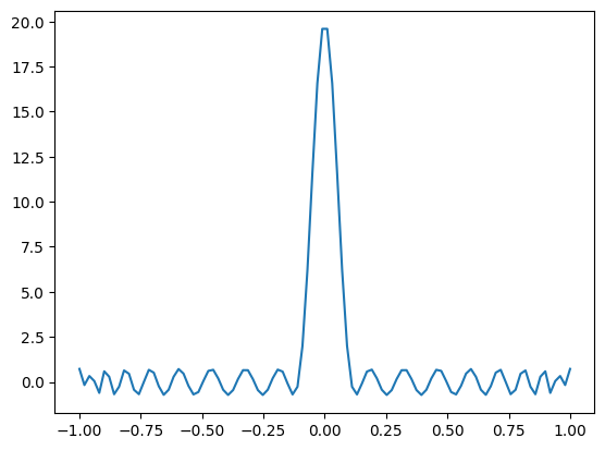

This polynomial needs to be converted to phases to use Quantum Signal Processing. For convenience, here are the phases for \(k=20\) and \(\Delta = 0.1\). At the end of the notebook, we show two ways to calculate the phases for a given polynomial.

# phases below are calculated using QSPPACK for n=20, delta = 0.1
phases = [ 0.76974538,  0.00646461, -0.00773143,  0.00908568, -0.01051591,  0.01200849,
          -0.01354772,  0.01511600, -0.01669402,  0.01826109, -0.01979540,  0.02127448,
          -0.02267559,  0.02397626, -0.02515479,  0.02619086, -0.02706603,  0.02776435,
          -0.02827282,  0.02858185, -0.02868552,  0.02858185, -0.02827282,  0.02776435,
          -0.02706603,  0.02619086, -0.02515479,  0.02397626, -0.02267559,  0.02127448,
          -0.01979540,  0.01826109, -0.01669402,  0.01511600, -0.01354772,  0.01200849,
          -0.01051591,  0.00908568, -0.00773143,  0.00646461,  0.76974538]

Hydrogen molecule example

We are going to prepare two different states using the phases above, as well as the Quantum Signal Processing circuit get_qsp_circuit_no_anc as defined in arXiv:2002.11649.

We are going to apply it to \(H_2\) in a STO-3G basis with the “scbk” qubit mapping.

from openfermion import get_sparse_operator
import numpy as np

from tangelo.molecule_library import mol_H2_sto3g
from tangelo.toolboxes.qubit_mappings.mapping_transform import fermion_to_qubit_mapping
from tangelo.linq.helpers.circuits.statevector import StateVector

fe_op = mol_H2_sto3g.fermionic_hamiltonian
qu_op = fermion_to_qubit_mapping(fe_op, "scbk", n_spinorbitals=4, n_electrons=2)

ham = get_sparse_operator(qu_op).toarray()
eigs, vecs = np.linalg.eigh(ham)
alpha = eigs[3]-eigs[0]

init_state = np.random.random(4)
init_state /= np.linalg.norm(init_state)

sv = StateVector(init_state)
init_circ = sv.initializing_circuit()

First excited state

We need to shift the Hamiltonian such that the desired eigenvalue (\(\lambda\)) is centered at zero and the spectral range is in [-1, 1]. This is done by defining

\(\tilde{H} = \frac{H-\lambda}{\alpha + \left|\lambda\right|}\)

where \(\alpha\) is the approximation to the spectral range, defined in the previous cell.

from tangelo.linq import Circuit, Gate, get_backend
from tangelo.toolboxes.circuits.qsp import get_qsp_circuit_no_anc
from tangelo.toolboxes.circuits.lcu import get_uprep_uselect, get_lcu_qubit_op_info

lamb = eigs[1]
# Shift Hamiltonian so that spectrum is in [-1, 1] and desired lambda is at 0
qu_op_tilde = (qu_op - lamb)/(alpha+abs(lamb))

# Generate LCU circuit that applies the Hamiltonian
uprep, uselect, qu_op_qs, m_qs, alpha = get_uprep_uselect(qu_op_tilde)
cua = uprep + uselect + uprep.inverse()

# Ancilla qubits
n_ancilla = len(m_qs) + 1

# Total number of qubits needed to apply algorithm
n_qubits = len(qu_op_qs) + n_ancilla

# Feed in LCU circuit to generate QSP circuit with phases for eigenvalue filtering
eig_filt_circ = get_qsp_circuit_no_anc(cua, m_qs, phases)

# Add the mesurement gates to the ancilla qubits for the application of the Linear Combination
# of Unitaries plus the extra qubit for the QSP
# Measure gates for LCU ancilla qubits
full_circuit = init_circ + eig_filt_circ + Circuit([Gate("MEASURE", m) for m in m_qs])
# Measure gate for the QSP qubit where the phases are applied
full_circuit += Circuit([Gate("MEASURE", m_qs[-1]+1)])

sim = get_backend()

f, sv = sim.simulate(full_circuit, desired_meas_result="0"*n_ancilla, return_statevector=True)
# Reorder statevector to "msq_first" if statevector in backend is "lsq_first"
if sim.backend_info()["statevector_order"] == "lsq_first":
    sv = np.reshape(sv, [2]*n_qubits).T.flatten()
# Pick out part of wavefunction that corresponds to "0000" on ancilla qubits
sv = np.reshape(sv, (2**4, 4))[0, :]
# Reorder statevector to correspond to openfermion ordering
sv = np.reshape(sv, (2,2)).T.flatten()

print(f'initial overlap = {abs(np.dot(vecs[:,1], init_state))}')
print(f'final overlap = {abs(np.dot(vecs[:,1], sv))}')

initial overlap = 0.18367656363390905
final overlap = 0.9887577317376988

Second excited state

We can then reapply the same approach to the second excited state.

lamb = eigs[2]
# Shift Hamiltonian so that spectrum is in [-1, 1] and desired lambda is at 0
qu_op_tilde = (qu_op - lamb)/(alpha+abs(lamb))

# Generate LCU circuit that applies the Hamiltonian
uprep, uselect, qu_op_qs, m_qs, alpha = get_uprep_uselect(qu_op_tilde)
cua = uprep + uselect + uprep.inverse()

# Ancilla qubits
n_ancilla = len(m_qs) + 1

# Total number of qubits needed to apply algorithm
n_qubits = len(qu_op_qs) + n_ancilla

# Feed in LCU circuit to generate QSP circuit with phases for eigenvalue filtering
eig_filt_circ = get_qsp_circuit_no_anc(cua, m_qs, phases)

full_circuit = init_circ + eig_filt_circ + Circuit([Gate("MEASURE", m) for m in m_qs])
full_circuit += Circuit([Gate("MEASURE", m_qs[-1]+1)])

sim = get_backend()

f, sv = sim.simulate(full_circuit, desired_meas_result="0"*n_ancilla, return_statevector=True)
# Reorder statevector to "msq_first" if statevector in backend is "lsq_first"
if sim.backend_info()["statevector_order"] == "lsq_first":
    sv = np.reshape(sv, [2]*n_qubits).T.flatten()
# Pick out part of wavefunction that corresponds to "0000" on ancilla qubits
sv = np.reshape(sv, (2**4, 4))[0, :]
# Reorder statevector to correspond to openfermion ordering
sv = np.reshape(sv, (2,2)).T.flatten()

print(f'initial overlap = {abs(np.dot(vecs[:,2], init_state))}')
print(f'final overlap = {abs(np.dot(vecs[:,2], sv))}')

initial overlap = 0.18413991077227115
final overlap = 0.9969619094421538

Code to generate phases

This section shows 2 options for converting a polynomial into phases, with either QSPPACK or pyqsp.

The cells are formatted in markdown as additional dependencies are required to run the following phase calculations, but the code below can be run once they are installed.

Using QSPPACK

from sympy.abc import x
from sympy import Rational
from sympy.functions.special.polynomials import chebyshevt

k = 20
# Necessary to work in exact representation for higher order polynomials
delta = Rational(delta)

def filter_func(x, delta, k):
    val = 0
    for i in range(k):
        arg = -1 + 2*((x**2-delta**2)/(1-delta**2))
        topk = chebyshevt(k, arg)
        arg = -1 + 2*(-delta**2/(1-delta**2))
        botk = chebyshevt(k, arg)
        val += topk/botk
    return val

We need to convert the filter_func polynomial to coefficients of expansion in Chebyshev polynomials to use with QSPPACK

# Use chebyshev interpolation ak=2/(n+1)*sum_{j=0}^n p(x_j)T_k(x_j), x_j = cos(\frac{2*j+1}{2*n+2}\pi)
poly = filter_func(x, delta, k).as_poly()

n = 2*k
xjs = np.zeros(n+1)
aks = np.zeros(n+1)
for j in range(n+1):
    xjs[j] = np.cos((2*j+1)/(2*n+2)*np.pi)

for ki in range(0, n+1, 2):
    aks[ki] = 0
    for j in range(n+1):
        aks[ki] += 2/(n+1)*poly.eval(xjs[j])*eval_chebyt(ki, xjs[j])

aks /= k*np.sqrt(2)
aks[0] /=2
aks = aks[0: n+1: 2]

We can then obtain the phases using oct2py (with octave installed) and the folder location of QSPPACK cloned from https://github.com/qsppack/QSPPACK.

from oct2py import octave

eps = 0.01
folder = 'path to QSPPACK'
octave.addpath(folder)
opts = octave.struct("criteria", eps)
phases, _ = octave.QSP_solver(aks, 0, opts, nout=2)

Using pyqsp

For \(k=20\), pyqsp with the laurent method works properly. However, it often fails for higher order polynomials. In that case, you can install tensorflow and use method=tf. It however seemed much slower than QSPPACK.

import pyqsp
from pyqsp import angle_sequence
from pyqsp.angle_sequence import AngleFindingError
from sympy.polys.polytools import primitive
from pyqsp.completion import CompletionError

# Compute phases for real part Cos(Ht) of Exp(iHt)
pg = pyqsp.poly.PolyCosineTX()
prefac, poly = primitive(filter_func(x, delta, k))
poly = poly.as_poly()
polydict = poly.as_dict()

coefs = np.zeros(2*k + 1, dtype=float)
for term, coeff in polydict.items():
    coefs[term[0]] = prefac*coeff/k/np.sqrt(2)

n_attempts = 100
method = 'laurent'
eps=0.01

for i in range(n_attempts):
    try:
        phases = angle_sequence.QuantumSignalProcessingPhases(
                coefs, eps=eps, suc=1-eps/10, method=method, tolerance=0.01)
    except (AngleFindingError, CompletionError):
        if i == n_attempts-1:
            raise RuntimeError("Real phases calculation failed, increase n_attempts or eps")
        else:
            print(f"Attempt {i+2} for the real coefficients")
    else:
        break