# Installation of tangelo if not already installed.
try:
    import tangelo
except ModuleNotFoundError:
    !pip install git+https://github.com/sandbox-quantum/Tangelo.git@develop --quiet

# Additional dependencies: pyscf (classical chemistry) and qulacs (quantum circuit simulation)
try:
    import qulacs
except ModuleNotFoundError:
!pip install pyscf qulacs --quietVQE with Tangelo
Tangelo provides various toolboxes, which can be leveraged to build quantum chemistry workflows relying on quantum computing. One example of such a workflow is the Variational Quantum Eigensolver (VQE). We provide an implementation of VQE that supports several options, and may provide valuable help in your research and applications.
This notebook assumes that you already have installed Tangelo in your Python environment, or have updated your Python path so that the imports can be resolved. If not, executing the cell below installs the minimal requirements for this notebook.
Table of contents:
1. Overview of VQE
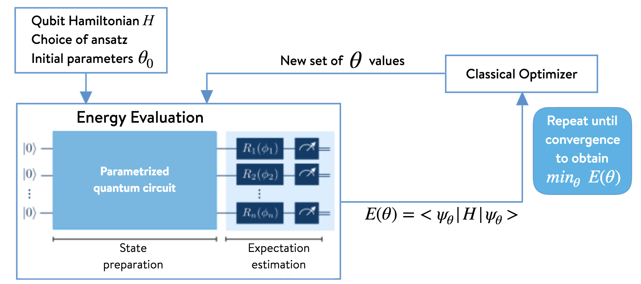
The Variational Quantum Eigensolver (VQE) [Peruzzo_et_al.,_2014, McClean_et_al.,_2015] has been introduced as a hybrid quantum–classical algorithm for simulating quantum systems. Some examples of quantum simulation using VQE include solving the molecular electronic Schrödinger equation and model systems in condensed matter physics (e.g., Fermi– and Bose–Hubbard models). In this notebook, we focus on VQE within the context of solving the molecular electronic structure problem for the ground-state energy of a molecular system. The second-quantized Hamiltonian of such a system, within the Born-Oppenheimer approximation, assumes the following form:
\[ \hat{H} = h_{\text{nuc}} + \sum\limits_{p,q} h^{p}_{q} a^{\dagger}_p a_q + \sum\limits_{p,q,r,s} h^{pq}_{rs} a^{\dagger}_p a^{\dagger}_q a_s a_r\nonumber \]
Here, \(h_{\text{nuc}}\) denotes the nuclear repulsion energy. In what follows below, we use the mean-field solution from Hartee-Fock (HF) self-consistent theory as our computational starting point. As such, the basis-orbitals and coefficients \(h_p^q\), \(h_{rs}^{pq}\), are evaluated in the basis of molecular orbitals from HF. The Hamiltonian is then transformed into the qubit basis (e.g., Jordan–Wigner, Bravyi–Kitaev). This means that it is expressed entirely in terms of operators acting on qubits:
\[ \hat{H} = h_{\text{nuc}} + \sum\limits_{\substack{p \\ \alpha}} h_{p}^{\alpha} \sigma_p^{\alpha} + \sum\limits_{\substack{p,q \\ \alpha,\beta}} h_{pq}^{\alpha\beta}\sigma_p^{\alpha}\otimes\sigma_{q}^{\beta} + \sum\limits_{\substack{p,q,r \\ \alpha,\beta,\gamma}}h_{pqr}^{\alpha\beta\gamma}\sigma_p^{\alpha}\otimes\sigma_{q}^{\beta}\otimes\sigma_r^{\gamma} + \ldots \nonumber \]
In this expression, the \(\sigma_p^\alpha\) are Pauli matrices (\(\alpha \in \{x,y,z\}\)), acting on the \(p\)-th qubit. We now consider a trial wavefunction ansatz \(\vert \Psi(\vec{\theta}) \rangle = U(\vec{\theta}) \vert 0 \rangle\) that depends on \(m\) parameters defining \(\vec{\theta}=(\theta_1, \theta_2, \ldots, \theta_m)\), which enter a unitary operator that acts on the reference (i.e., mean-field) state \(\vert 0 \rangle\). The variational principle dictates that we can minimize the expectation value of the Hamiltonian,
\[ E = \min\limits_{\vec{\theta}} \frac{\langle \Psi(\vec{\theta}) \vert \hat{H} \vert \Psi(\vec{\theta}) \rangle}{\langle \Psi(\vec{\theta}) \vert \Psi(\vec{\theta}) \rangle} \geq E_{\text{gs}}\nonumber \]
to determine the optimal set of variational parameters. The energy thus computed will be an upper bound to the true ground-state energy \(E_{\text{gs}}\). Once a suitable variational trial ansatz has been chosen (e.g., a unitary coupled-cluster ansatz, a heuristic ansatz), we must provide a suitable set of initial guess parameters. If our ansatz is defined in the formalism of second-quantization, we must also transform it into the qubit basis before proceeding. We must also apply other approximations (e.g., Trotter–Suzuki) to render it amenable for translation into a quantum circuit. The resulting qubit form of the ansatz can then be translated into a quantum circuit and, thus, able to be implemented on quantum hardware. Once the initial state has been prepared using a quantum circuit, energy measurements are performed using quantum hardware or an appropriate simulation tool. The energy value obtained is the sum of the measurements of the expectation values of each of the terms that contribute to the Hamiltonian (assuming the wavefunction has been normalized to unity):
\[ E = \langle \Psi(\vec{\theta}) \vert \hat{H} \vert \Psi(\vec{\theta}) \rangle =\langle\hat{H}\rangle = h_{\text{nuc}} + \sum_{\substack{p \\ \alpha}} h_{p}^{\alpha} \langle\sigma_p^{\alpha}\rangle + \sum_{\substack{p,q \\ \alpha,\beta}} h_{pq}^{\alpha\beta}\langle\sigma_p^{\alpha}\otimes\sigma_{q}^{\beta}\rangle + \sum_{\substack{p,q,r \\ \alpha,\beta,\gamma}}h_{pqr}^{\alpha\beta\gamma}\langle\sigma_p^{\alpha}\otimes\sigma_{q}^{\beta}\otimes\sigma_r^{\gamma}\rangle + \ldots \nonumber \]
The computed energy is then input to a classical optimizer in order to find a new set of variational parameters, which are then used to prepare a new state (i.e., a quantum circuit) on the quantum hardware. The process is repeated until convergence. The algorithm is illustrated below.
2. VQESolver class
In the following, we will demonstrate various features of the VQESolver class using a simple H2 molecule, defined with the SecondQuantizedMolecule class. This molecule is built below:
from tangelo import SecondQuantizedMolecule

H2 = [('H', (0, 0, 0)),('H', (0, 0, 0.74137727))]
mol_H2 = SecondQuantizedMolecule(H2, q=0, spin=0, basis="sto-3g")
The VQESolver class implements the VQE electronic structure solver and can be found under the electronic_structure_solver module, along with FCISolver and CCSDSolver, which are classical electronic structure solvers that we will only use here to compare reference results.
In essence, VQE can simply be run using these 3 steps - Instantiate the VQESolver object with the desired options and molecule - Call the build method to construct the objects (e.g. ansatz circuit) required to perform VQE - Call the simulate method to execute the VQE algorithm
In this section, we will go through these 3 steps, and introduce you to other useful functionalities.
VQESolver object instantiation
The VQESolver class can be instantiated by passing a dictionary. Currently, the molecule field must be provided, and everything else is optional. In the future, this constraint may be relaxed to support different workflows, relying directly on a precomputed qubit operator for example.
In the cell below, we initiate a VQESolver object with this molecule, and display the various attributes of the objects. Notice that some of them have been filled with default values.
from tangelo.algorithms import VQESolver

vqe_options = {"molecule": mol_H2}
vqe_solver = VQESolver(vqe_options)
vars(vqe_solver)
{'molecule': SecondQuantizedMolecule(xyz=[('H', (0.0, 0.0, 0.0)), ('H', (0.0, 0.0, 0.74137727))], q=0, spin=0, n_atoms=2, n_electrons=2, n_min_orbitals=8, basis='sto-3g', ecp={}, symmetry=False, mf_energy=-1.1166856303994788, mo_energies=array([-0.5779842, 0.6697221]), mo_occ=array([2., 0.]), mean_field=<pyscf.scf.hf.RHF object at 0x7fa46c643040>, n_mos=2, n_sos=4, active_occupied=[0], frozen_occupied=[], active_virtual=[1], frozen_virtual=[]),
'qubit_mapping': 'jw',
'ansatz': <BuiltInAnsatze.UCCSD: 0>,
'optimizer': <bound method VQESolver._default_optimizer of <tangelo.algorithms.variational.vqe_solver.VQESolver object at 0x7fa46e659910>>,
'initial_var_params': None,
'backend_options': {'target': None, 'n_shots': None, 'noise_model': None},
'penalty_terms': None,
'deflation_circuits': [],
'deflation_coeff': 1,
'ansatz_options': {},
'up_then_down': False,
'qubit_hamiltonian': None,
'verbose': False,
'ref_state': None,
'reference_circuit': <tangelo.linq.circuit.Circuit at 0x7fa429202220>,
'default_backend_options': {'target': None,
'n_shots': None,
'noise_model': None},
'optimal_energy': None,
'optimal_var_params': None,
'builtin_ansatze': {<BuiltInAnsatze.HEA: 3>,
<BuiltInAnsatze.ILC: 9>,
<BuiltInAnsatze.QCC: 6>,
<BuiltInAnsatze.QMF: 5>,
<BuiltInAnsatze.UCC1: 1>,
<BuiltInAnsatze.UCC3: 2>,
<BuiltInAnsatze.UCCGD: 8>,
<BuiltInAnsatze.UCCSD: 0>,
<BuiltInAnsatze.UpCCGSD: 4>,
<BuiltInAnsatze.VSQS: 7>}}Our object’s attributes have been populated using the dictionary provided by the user, and default values for the fields that had not been specified in there. Among these attributes, you will see a number of them related to classical optimization, ansatz circuits, qubit mappings or complementary information regarding the molecular system.
The VQESolver class has several methods that are relevant to us, we’ll go through them one by one.
VQESolver.build
This method builds all the internal objects required by VQE, based on the options provided during object instantiation. It will build the mean-field if necessary, the fermionic and qubit hamiltonians corresponding to your molecular system, as well as the ansatz circuit (for default values of variational parameters if none have been provided so far), and the backend performing quantum circuit simulation or execution (a classical simulator or quantum processor).
After we run build, we can see that a number of objects have been built and are now populating the attributes of our VQESolver object.
vqe_solver.build()
vars(vqe_solver)
{'molecule': SecondQuantizedMolecule(xyz=[('H', (0.0, 0.0, 0.0)), ('H', (0.0, 0.0, 0.74137727))], q=0, spin=0, n_atoms=2, n_electrons=2, n_min_orbitals=8, basis='sto-3g', ecp={}, symmetry=False, mf_energy=-1.1166856303994788, mo_energies=array([-0.5779842, 0.6697221]), mo_occ=array([2., 0.]), mean_field=<pyscf.scf.hf.RHF object at 0x7fa46c643040>, n_mos=2, n_sos=4, active_occupied=[0], frozen_occupied=[], active_virtual=[1], frozen_virtual=[]),
'qubit_mapping': 'jw',
'ansatz': <tangelo.toolboxes.ansatz_generator.uccsd.UCCSD at 0x7fa42916e760>,
'optimizer': <bound method VQESolver._default_optimizer of <tangelo.algorithms.variational.vqe_solver.VQESolver object at 0x7fa46e659910>>,
'initial_var_params': [2e-05, 0.03632416060255425],
'backend_options': {'target': None, 'n_shots': None, 'noise_model': None},
'penalty_terms': None,
'deflation_circuits': [],
'deflation_coeff': 1,
'ansatz_options': {},
'up_then_down': False,
'qubit_hamiltonian': (-0.09883484730799569+0j) [] +
(-0.045321883918106265+0j) [X0 X1 Y2 Y3] +
(0.045321883918106265+0j) [X0 Y1 Y2 X3] +
(0.045321883918106265+0j) [Y0 X1 X2 Y3] +
(-0.045321883918106265+0j) [Y0 Y1 X2 X3] +
(0.17120123806595938+0j) [Z0] +
(0.16862327595071586+0j) [Z0 Z1] +
(0.12054612740556847+0j) [Z0 Z2] +
(0.16586801132367474+0j) [Z0 Z3] +
(0.1712012380659594+0j) [Z1] +
(0.16586801132367474+0j) [Z1 Z2] +
(0.12054612740556847+0j) [Z1 Z3] +
(-0.22279639651093203+0j) [Z2] +
(0.17434948757007068+0j) [Z2 Z3] +
(-0.22279639651093203+0j) [Z3],
'verbose': False,
'ref_state': None,
'reference_circuit': <tangelo.linq.circuit.Circuit at 0x7fa429202220>,
'default_backend_options': {'target': None,
'n_shots': None,
'noise_model': None},
'optimal_energy': None,
'optimal_var_params': None,
'builtin_ansatze': {<BuiltInAnsatze.HEA: 3>,
<BuiltInAnsatze.ILC: 9>,
<BuiltInAnsatze.QCC: 6>,
<BuiltInAnsatze.QMF: 5>,
<BuiltInAnsatze.UCC1: 1>,
<BuiltInAnsatze.UCC3: 2>,
<BuiltInAnsatze.UCCGD: 8>,
<BuiltInAnsatze.UCCSD: 0>,
<BuiltInAnsatze.UpCCGSD: 4>,
<BuiltInAnsatze.VSQS: 7>},
'backend': <tangelo.linq.simulator.Simulator at 0x7fa42916e7c0>}In particular we notice:
- qubit Hamiltonian: the qubit operator used for computing the expectation value in the energy estimation step of VQE
- backend is a
Simulatorobject that was defined in a submodule calledlinq, allowing us to define how a quantum circuit should be run. Currently, the default option is to run using an exact simulation (no noise) using thequlacsclassical simulator. - ansatz: is now an object that implements the UCCSD ansatz. We go into more details about builtin and custom ansatze in a separate notebook. For now, it is useful to notice that one can peek at the UCCSD quantum circuit that was built, or the value of the variational parameters for this ansatz. This quantum circuit is in the format implemented in
linq.
print(f"Variational parameters: {vqe_solver.ansatz.var_params}\n")
print(vqe_solver.ansatz.circuit)
Variational parameters: [2e-05, 0.03632416060255425]
Circuit object. Size 158
X target : [0]
X target : [1]
RX target : [0] parameter : 1.5707963267948966
H target : [2]
CNOT target : [1] control : [0]
CNOT target : [2] control : [1]
RZ target : [2] parameter : 2e-05 (variational)
CNOT target : [2] control : [1]
CNOT target : [1] control : [0]
H target : [2]
RX target : [0] parameter : -1.5707963267948966
H target : [0]
RX target : [2] parameter : 1.5707963267948966
CNOT target : [1] control : [0]
CNOT target : [2] control : [1]
RZ target : [2] parameter : 12.566350614359173 (variational)
CNOT target : [2] control : [1]
CNOT target : [1] control : [0]
RX target : [2] parameter : -1.5707963267948966
H target : [0]
RX target : [1] parameter : 1.5707963267948966
H target : [3]
CNOT target : [2] control : [1]
CNOT target : [3] control : [2]
RZ target : [3] parameter : 2e-05 (variational)
CNOT target : [3] control : [2]
CNOT target : [2] control : [1]
H target : [3]
RX target : [1] parameter : -1.5707963267948966
H target : [1]
RX target : [3] parameter : 1.5707963267948966
CNOT target : [2] control : [1]
CNOT target : [3] control : [2]
RZ target : [3] parameter : 12.566350614359173 (variational)
CNOT target : [3] control : [2]
CNOT target : [2] control : [1]
RX target : [3] parameter : -1.5707963267948966
H target : [1]
RX target : [0] parameter : 1.5707963267948966
RX target : [1] parameter : 1.5707963267948966
RX target : [2] parameter : 1.5707963267948966
H target : [3]
CNOT target : [1] control : [0]
CNOT target : [2] control : [1]
CNOT target : [3] control : [2]
RZ target : [3] parameter : 0.018162080301277125 (variational)
CNOT target : [3] control : [2]
CNOT target : [2] control : [1]
CNOT target : [1] control : [0]
H target : [3]
RX target : [2] parameter : -1.5707963267948966
RX target : [1] parameter : -1.5707963267948966
RX target : [0] parameter : -1.5707963267948966
RX target : [0] parameter : 1.5707963267948966
H target : [1]
RX target : [2] parameter : 1.5707963267948966
RX target : [3] parameter : 1.5707963267948966
CNOT target : [1] control : [0]
CNOT target : [2] control : [1]
CNOT target : [3] control : [2]
RZ target : [3] parameter : 12.548208534057895 (variational)
CNOT target : [3] control : [2]
CNOT target : [2] control : [1]
CNOT target : [1] control : [0]
RX target : [3] parameter : -1.5707963267948966
RX target : [2] parameter : -1.5707963267948966
H target : [1]
RX target : [0] parameter : -1.5707963267948966
H target : [0]
H target : [1]
RX target : [2] parameter : 1.5707963267948966
H target : [3]
CNOT target : [1] control : [0]
CNOT target : [2] control : [1]
CNOT target : [3] control : [2]
RZ target : [3] parameter : 12.548208534057895 (variational)
CNOT target : [3] control : [2]
CNOT target : [2] control : [1]
CNOT target : [1] control : [0]
H target : [3]
RX target : [2] parameter : -1.5707963267948966
H target : [1]
H target : [0]
H target : [0]
RX target : [1] parameter : 1.5707963267948966
RX target : [2] parameter : 1.5707963267948966
RX target : [3] parameter : 1.5707963267948966
CNOT target : [1] control : [0]
CNOT target : [2] control : [1]
CNOT target : [3] control : [2]
RZ target : [3] parameter : 12.548208534057895 (variational)
CNOT target : [3] control : [2]
CNOT target : [2] control : [1]
CNOT target : [1] control : [0]
RX target : [3] parameter : -1.5707963267948966
RX target : [2] parameter : -1.5707963267948966
RX target : [1] parameter : -1.5707963267948966
H target : [0]
RX target : [0] parameter : 1.5707963267948966
H target : [1]
H target : [2]
H target : [3]
CNOT target : [1] control : [0]
CNOT target : [2] control : [1]
CNOT target : [3] control : [2]
RZ target : [3] parameter : 0.018162080301277125 (variational)
CNOT target : [3] control : [2]
CNOT target : [2] control : [1]
CNOT target : [1] control : [0]
H target : [3]
H target : [2]
H target : [1]
RX target : [0] parameter : -1.5707963267948966
RX target : [0] parameter : 1.5707963267948966
RX target : [1] parameter : 1.5707963267948966
H target : [2]
RX target : [3] parameter : 1.5707963267948966
CNOT target : [1] control : [0]
CNOT target : [2] control : [1]
CNOT target : [3] control : [2]
RZ target : [3] parameter : 0.018162080301277125 (variational)
CNOT target : [3] control : [2]
CNOT target : [2] control : [1]
CNOT target : [1] control : [0]
RX target : [3] parameter : -1.5707963267948966
H target : [2]
RX target : [1] parameter : -1.5707963267948966
RX target : [0] parameter : -1.5707963267948966
H target : [0]
RX target : [1] parameter : 1.5707963267948966
H target : [2]
H target : [3]
CNOT target : [1] control : [0]
CNOT target : [2] control : [1]
CNOT target : [3] control : [2]
RZ target : [3] parameter : 0.018162080301277125 (variational)
CNOT target : [3] control : [2]
CNOT target : [2] control : [1]
CNOT target : [1] control : [0]
H target : [3]
H target : [2]
RX target : [1] parameter : -1.5707963267948966
H target : [0]
H target : [0]
H target : [1]
H target : [2]
RX target : [3] parameter : 1.5707963267948966
CNOT target : [1] control : [0]
CNOT target : [2] control : [1]
CNOT target : [3] control : [2]
RZ target : [3] parameter : 12.548208534057895 (variational)
CNOT target : [3] control : [2]
CNOT target : [2] control : [1]
CNOT target : [1] control : [0]
RX target : [3] parameter : -1.5707963267948966
H target : [2]
H target : [1]
H target : [0]
:warning: If you are not familiar with the
linqsubmodule, we recommend you check at some point the tutorial covering the basics. You can however keep going through this notebook without issues.
VQE.simulate
After VQE.build has been run, we now have all the objects needed to run the VQE algorithm, which consists in a classical optimization loop over an energy estimation function. This energy estimation is obtained by computing the expectation value of our qubit Hamiltonian, with regards to the variational ansatz circuit.
The classical loop is driven by the selected optimizer (we’ll see a bit later how you can choose that), as well as the initial variational parameters.
This method returns the optimal energy computed during the optimization process. As a byproduct, the attributes optimal_energy and optimal_var_params of our VQESolver object have been updated. If you have turned on the verbose option, your output will print more information about energy during the optimization process.
energy_vqe = vqe_solver.simulate()
print(f"\nOptimal energy: \t {energy_vqe}")
print(f"Optimal parameters: \t {vqe_solver.optimal_var_params}")
Optimal energy:      -1.1372704157729143
Optimal parameters:      [-5.4412497e-05  5.6522190e-02]
That’s it, we ran VQE ! We can quickly check whether or not it did well on this system, with the options we picked: let’s compare that to what classical approaches like CCSD or FCI can do. UCCSD captures single and double excitations, and should be exact for a system like H2, assuming the classical optimization of the variational parameters was succesful.
The CCSDSolver and FCISolver objects have a slightly different interface than VQESolver but are very straightforward. As we can see, the energies are in agreement, indicating that VQE did a good job.
from tangelo.algorithms import FCISolver, CCSDSolver

fci_solver = FCISolver(mol_H2)
energy_fci = fci_solver.simulate()

ccsd_solver = CCSDSolver(mol_H2)
energy_ccsd = ccsd_solver.simulate()

print(f"FCI energy: \t {energy_fci}")
print(f"CCSD energy: \t {energy_ccsd}")
print(f"VQE energy: \t {energy_vqe}")
FCI energy: -1.1372704220924397
CCSD energy: -1.1372704220914702
VQE energy: -1.1372704157729143VQE.energy_estimation
The VQE.energy_estimation is a convenient method that allows you to run a single energy estimation, for some given variational parameters.
This would allow you to compare maybe different (initial?) variational parameters, or could be used to rebuild the underlying ansatz circuit for specific values of the variational parameters, without involving the classical optimization.
The UCCSD ansatz supports a few “shortcut” keywords for some parameters, such as “MP2”, “ones” or “random” (don’t hesitate to explore the ansatz attribute of your VQESolver object, in particular the n_var_params value). We can compare the energy they return: we see below that the mp2 parameters are a much better pick as initial parameters, but not as good as the optimal ones found by simulate earlier.
Since this method builds the ansatz circuit for the input parameter, you can then grab the corresponding circuit. If you know the optimal parameters (from maybe a previous call to simulate), you can then grab the optimal circuit. Check out the linq tutorials to get an idea of how you could explore, export and send this circuit to a collaborator or a compute backend !
# Compare energies associated to different variational parameters
energy = vqe_solver.energy_estimation("ones")
print(f"{energy:.7f} (params = {vqe_solver.ansatz.var_params})")

energy = vqe_solver.energy_estimation("MP2")
print(f"{energy:.7f} (params = {vqe_solver.ansatz.var_params})")

energy = vqe_solver.energy_estimation(vqe_solver.optimal_var_params)
print(f"{energy:.7f} (params = {vqe_solver.ansatz.var_params})")

# You can retrieve the circuit corresponding to the last parameters you have used
optimal_circuit = vqe_solver.ansatz.circuit
-0.3369215 (params = [1. 1.])
-1.1346304 (params = [2e-05, 0.03632416060255425])
-1.1372704 (params = [-5.4412497e-05 5.6522190e-02])VQE.get_resources
What we can or can’t simulate on backends today (may they be classical simulators or QPUs) is essentially driven by resource requirements. Metrics that correlate to the number of qubits, gates or measurements an algorithm would require to be performed accurately tell a lot about its feasibility on NISQ hardware, and can be used to compare different approaches, without having to actually do any simulation.
This method is able to grab the relevant information for our VQESolver by peeking into the underlying ansatz and qubit Hamiltonian objects. The information you receive is tied to the options you picked for VQE, and may not be true for all sets of variational parameters, depending on how the ansatz circuit is built, and potential optimizations done in the future to the circuit. We also return the number of variational parameters in VQE, as the difficulty of classical optimization plays an important role in the success of the algorithm.
More features for estimating the number of measurements to run an experiment with a given accuracy are on our roadmap.
Here’s what our current example returns:
resources = vqe_solver.get_resources()
print(resources)
{'qubit_hamiltonian_terms': 15, 'circuit_width': 4, 'circuit_gates': 158, 'circuit_2qubit_gates': 64, 'circuit_var_gates': 12, 'vqe_variational_parameters': 2}VQE.get_rdm
The get_rdm method enables us to compute the one- and two-electron Reduced Density Matrices (RDM) using the ansatz circuit previously built by VQESolver, for some input variational parameters. This can come in handy, and is in particular used by the DMET problem decomposition technique, further detailed in another notebook.
Below, we compute these RDMs using the optimal variational parameters found by a previous call to simulate, and only print the one-electron RDM.
onerdm, twordm = vqe_solver.get_rdm(vqe_solver.optimal_var_params)
print(onerdm)
[[1.97455062+0.j 0. +0.j]
[0. +0.j 0.02544938+0.j]]3. Option: frozen orbitals
The VQESolver class supports a frozen_orbitals option, allowing a user to pass either a list of indices (integers) referring to the orbitals to freeze, or a single integer indicating that all orbitals up to that index (excluded) must be frozen. For instance, just passing 3 would be equivalent to passing [0, 1, 2].
Internally, this information is parsed and allows us to track which orbitals are active or frozen and occupied or virtual, through an object carrying molecular data which is an attribute of the VQESolver. By default, the option “frozen_core” is selected. If this string is detected, the function tangelo.toolboxes.molecular_computation.frozen_orbitals.get_frozen_core is called. It takes a Molecule or a SecondQuantizedMolecule object and returns an integer corresponding to the number of low-energy orbitals. In short, no orbital for each period 1 element, one orbital for each period 2 element and five orbitals for each period 3 element are summed up and frozen in the subsequent calculation. It is important to emphasize that this option does nothing if a custom qubit Hamiltonian is provided instead of a molecule.
Let’s have a look at this quickly, taking a H4 molecule in sto-3g basis as an example. We can compare the results provided by VQE to our classical CCSD solver, which also support frozen orbitals with a slightly different interface.
H4 = [["H", [0.7071067811865476, 0.0, 0.0]], ["H", [0.0, 0.7071067811865476, 0.0]],
      ["H", [-1.0071067811865476, 0.0, 0.0]], ["H", [0.0, -1.0071067811865476, 0.0]]]

mol_H4 = SecondQuantizedMolecule(H4, q=0, spin=0, basis="sto-3g", frozen_orbitals=[0, 3])
vqe_options = {"molecule": mol_H4}
vqe_solver_h4_frozen = VQESolver(vqe_options)
vqe_solver_h4_frozen.build()
energy_vqe_h4_frozen = vqe_solver_h4_frozen.simulate()
print(f"VQE energy: \t {energy_vqe_h4_frozen}")
ccsd_solver = CCSDSolver(mol_H4)
energy_ccsd_h4_frozen = ccsd_solver.simulate()
print(f"CCSD energy: \t {energy_ccsd_h4_frozen}")
print("\n", vqe_solver_h4_frozen.get_resources())VQE energy: -1.8943598012228877
CCSD energy: -1.894360237665742
{'qubit_hamiltonian_terms': 15, 'circuit_width': 4, 'circuit_gates': 158, 'circuit_2qubit_gates': 64, 'circuit_var_gates': 12, 'vqe_variational_parameters': 2}Frozen orbitals offer a trade-off between resource requirements and accuracy. By freezing orbitals that seem not to contribute significantly to the computation, we may drastically reduce resource requirements. In this example, we sacrificed a noticeable amount of accuracy but also drastically reduced resource requirements and ended up with a formulation that was much easier to solve. Notice how simulate takes longer to execute here, and compare both energies and resource requirements to the previous cell.
mol_H4 = SecondQuantizedMolecule(H4, q=0, spin=0, basis="sto-3g", frozen_orbitals=None)

vqe_options = {"molecule": mol_H4}
vqe_solver_h4 = VQESolver(vqe_options)
vqe_solver_h4.build()

energy_vqe_h4 = vqe_solver_h4.simulate()
print(f"VQE energy: \t {energy_vqe_h4}")
print("\n", vqe_solver_h4.get_resources())
VQE energy: -1.9778372805046642
{'qubit_hamiltonian_terms': 185, 'circuit_width': 8, 'circuit_gates': 2692, 'circuit_2qubit_gates': 1312, 'circuit_var_gates': 160, 'vqe_variational_parameters': 14}4. Option: ansatz and qubit mapping
VQE relies on a qubit mapping in order to encode the fermionic-Hamiltonian into a spin-Hamiltonian which can be expressed natively on quantum hardware. This enables us to represent the occupation of fermionic orbital basis states in terms of the internal state of a collection of qubits. Meanwhile, the ansatz drives what portion of the Hilbert space can be explored by VQE, as we change the values of the variational parameters.
We can choose from a number of built-in ansatze (UCCSD, UCC1, UCC3…) and qubit mappings (Jordan-Wigner, Bravyi-Kitaev, symmetry-conserving Bravyi-Kitaev). In the previous examples, the default options for these two entities were selected. You may have noticed that the qubit mapping was Jordan-Wigner ('jw'), and the ansatz was UCCSD (Ansatze.UCCSD).
The choice of qubit mapping and ansatz impacts resource requirements but also accuracy. Designing “shallow” ansatze with low resource requirements that yield accurate results is an active topic of research.
Below, we show how the qubit mapping impacts our example on H2 using the UCCSD ansatz. Notice the difference in resource requirements, classical optimization, and the difference in accuracy.
from tangelo.algorithms import BuiltInAnsatze as Ansatze

# VQE-UCCSD on H2 with different qubit mappings
for qm in ['jw', 'bk', 'scbk']:
    vqe_options = {"molecule": mol_H2, "ansatz": Ansatze.UCCSD, "qubit_mapping": qm}
    vqe_solver = VQESolver(vqe_options)
    vqe_solver.build()
    vqe_solver.simulate()
    print("\n", vqe_solver.get_resources(), "\n")
 {'qubit_hamiltonian_terms': 15, 'circuit_width': 4, 'circuit_gates': 158, 'circuit_2qubit_gates': 64, 'circuit_var_gates': 12, 'vqe_variational_parameters': 2}


 {'qubit_hamiltonian_terms': 15, 'circuit_width': 4, 'circuit_gates': 107, 'circuit_2qubit_gates': 46, 'circuit_var_gates': 12, 'vqe_variational_parameters': 2}


 {'qubit_hamiltonian_terms': 5, 'circuit_width': 2, 'circuit_gates': 22, 'circuit_2qubit_gates': 4, 'circuit_var_gates': 4, 'vqe_variational_parameters': 2}
/home/alex/Codes/Tangelo/tangelo/toolboxes/qubit_mappings/statevector_mapping.py:149: RuntimeWarning: Symmetry-conserving Bravyi-Kitaev enforces all spin-up followed by all spin-down ordering.
  warnings.warn("Symmetry-conserving Bravyi-Kitaev enforces all spin-up followed by all spin-down ordering.", RuntimeWarning)
:warning: Each ansatz works differently, or may not be compatible with all qubit mappings. We encourage you to check out the documentation. In particular, how the
Ansatzclass work and how to implement your own custom ansatz into VQE is covered in a separate notebookvqe_custom_ansatz_hamiltonian.ipynb.
We can also try using the restricted UCC ansatze UCC1 and UCC3 to solve this problem:
# VQE-UCCSD on H2 with ansatze UCC1 and UCC3
for az in [Ansatze.UCC1, Ansatze.UCC3]:
    vqe_options = {"molecule": mol_H2, "ansatz": az, "up_then_down": True}
    vqe_solver = VQESolver(vqe_options)
    vqe_solver.build()
    vqe_solver.simulate()
    print("\n", vqe_solver.get_resources(), "\n")
 {'qubit_hamiltonian_terms': 15, 'circuit_width': 4, 'circuit_gates': 17, 'circuit_2qubit_gates': 6, 'circuit_var_gates': 1, 'vqe_variational_parameters': 1}


 {'qubit_hamiltonian_terms': 15, 'circuit_width': 4, 'circuit_gates': 23, 'circuit_2qubit_gates': 8, 'circuit_var_gates': 3, 'vqe_variational_parameters': 3}
5. Option: classical optimization
You also have full control over the classical optimization strategy you wish to follow. Earlier, we showed how the initial_var_params attribute of the VQESolver class could be used in different ways: check out the implementation of your ansatz object to see what is supported.
Users can also provide their own optimizer, which will be called in VQESolver.simulate and be passed a handle to the VQESolver.energy_estimation function and the initial variational parameters. Below, we decide to use the COBYLA optimizer from scipy:
It is required that both the resulting function value and resulting parameters (result.fun and result.x respectively for the example below) are returns for the user defined function. This allows easy access after optimization to the optimal energy from vqe_solver.optimal_energy, and optimal parameters from vqe_solver.optimal_var_params.
def cobyla_optimizer(func, var_params):
    from scipy.optimize import minimize
    result = minimize(func, var_params, method="COBYLA", options={"disp": True, "maxiter": 100, 'rhobeg':0.1})

    print(f"\tOptimal UCCSD energy: {result.fun}")
    print(f"\tOptimal UCCSD variational parameters: {result.x}")
    print(f"\tNumber of Function Evaluations : {result.nfev}")
    return result.fun, result.x

# Use "optimizer" and "initial_var_params" to customize your classical optimization
vqe_options = {"molecule": mol_H2, "optimizer": cobyla_optimizer, "initial_var_params": [1., 2.]}
vqe_solver = VQESolver(vqe_options)
vqe_solver.build()
optimal_energy = vqe_solver.simulate()
Optimal UCCSD energy: -1.1372704174429256
Normal return from subroutine COBYLA
NFVALS = 36 F =-1.137270E+00 MAXCV = 0.000000E+00
X = 1.570763E+00 2.412707E+00
Optimal UCCSD variational parameters: [1.57076299 2.41270658]
Number of Function Evaluations : 366. Option: compute backend
The VQESolver class relies on the linq submodule in order to simulate your quantum circuits.
For more information about the backend attribute of your VQE_Solver object, of type tangelo.linq.Simulator, we recommend you check the linq tutorial notebooks.
This object allows you to pick from a number of different classical simulators, with significantly different performance, some supporting noisy simulation. The parameters n_shots introduces statistical noise in the computation, which correlates to accuracy of energy estimation, while noise_model enables us to model noise in the circuit to an extent. These parameters are provided to enable the modeling of experiments that may be closer to the behaviour of quantum hardware.
Below, we specify that we’d like our VQESolver to use the simulator from the cirq Python package as a backend, and leave the two other parameters to None to signify that we want the simulation to be exact.
my_backend_options = {"target": "cirq", "n_shots": None, "noise_model": None}
vqe_options = {"molecule": mol_H2, "backend_options": my_backend_options, "verbose": True}
vqe_solver = VQESolver(vqe_options)
vqe_solver.build()

for term, coef in vqe_solver.qubit_hamiltonian.terms.items():
    vqe_solver.qubit_hamiltonian.terms[term] = coef.real

vqe_solver.simulate()

opt_energy = vqe_solver.optimal_energy
opt_params = vqe_solver.optimal_var_params
VQESolver optimization results:
Optimal VQE energy: -1.1372704157729134
Optimal VQE variational parameters: [-5.44125627e-05 5.65221900e-02]
Number of Iterations : 3
Number of Function Evaluations : 10
Number of Gradient Evaluations : 3Running VQE on a noisy backend is a challenge in itself, and it is hard to predict what will be the behavior on the algorithm when the output is based on drawing shots (samples), which reflects the probabilistic nature of a quantum processor.
What optimizer should be used for a noisy function? How does it correlate with the number of shots (samples) we need to gather for each energy estimation ? Is there any hope for VQE to be useful on a quantum computer ? All of these are open questions.
Below, we illustrate how one can see that the amount of shots (samples) taken for energy estimation leads to better accuracy:
my_backend_options = {"target": "qulacs", "n_shots": 1, "noise_model": None}
vqe_options = {"molecule": mol_H2, "backend_options": my_backend_options}
vqe_solver = VQESolver(vqe_options)
vqe_solver.build()

for n_shots in [10**2, 10**4, 10**6]:
    vqe_solver.backend.n_shots = n_shots
    energy = vqe_solver.energy_estimation(opt_params)
    print(f"Energy estimation with {n_shots:.1E} shots = {energy} \t(Error: {abs(energy - opt_energy):.2E})")
Energy estimation with 1.0E+02 shots = -1.1335574814374392 (Error: 3.71E-03)
Energy estimation with 1.0E+04 shots = -1.1358696314459025 (Error: 1.40E-03)
Energy estimation with 1.0E+06 shots = -1.1372051734252862 (Error: 6.52E-05)Closing words
This concludes our overview of VQESolver. Due to the complexity of the topic, we did not explore in details some of the underlying objects it relies on, such as the ansatz object and the backend object.
For a more in-depth discussion on these objects, please refer to the documentation and check out the other notebooks we have in this folder, or maybe the linq notebooks.