# Pretty printer for more readable outputs
import pprint
pp = pprint.PrettyPrinter(width=160, compact=False, indent=1)
from pprint import pprint

# Installation of tangelo if not already installed.
try:
    import tangelo
except ModuleNotFoundError:
!pip install git+https://github.com/sandbox-quantum/Tangelo.git@develop --quietEnd-to-end Quantum Chemistry Workflow on Quantum Hardware with Tangelo
Quantum computing is a nascent field, and we have barely started to explore its applications. In order to revolutionize fields such as quantum chemistry, the community has to face challenges in both algorithms design and quantum hardware development. A major undertaking is designing approaches ensuring satisfying accuracy, while keeping computing resource requirements within the capabilities of Noisy Intermediate Scale Quantum (NISQ) devices to solve exciting problems.
This quantum SDK was designed to support our exploration with this goal in mind, and enables us to build our own end-to-end workflows by providing building-blocks from various toolboxes, and algorithms.
The present notebook attempts to provide a step-by-step tutorial from starting with an expression of a molecule all the way to post-processing the results coming from the quantum hardware to obtain successful final results. More specifically we cover the following steps:
Table of contents:
- 1. Setting up your environment
- 2. Introducing our use case
- 3. Representing the input molecular data
- 4. Calculating reference energy with classical solvers
- 5. Exploring approaches using resource estimation and problem decomposition
- 6. Validating the desired approach with simulators
- 7. Minimizing the amount of resources needed for the hardware experiment
- 8. Submitting an experiment to a quantum device
- 9. Post-processing and error-mitigation of raw hardware results
- 10. Closing words
In this notebook, we illustrate how Tangelo can be used to re-enact one of our recent successful quantum chemistry experiments, done in collaboration with Dow and IonQ [Kawashima et al., 2021]. This experiment features an electronic system that could not be realistically solved with a heads-on approach on an existing quantum computer, yet produced great experimental results by combining the DMET problem decomposition technique [Knizia et al., 2013a and Knizia et al., 2013b] with the VQE algorithm [Kassal et al., 2011, Peruzzo et al., 2014 and Cao et al., 2019] and error-mitigation techniques [Bharti et al., 2021], running on an ion-trap-based quantum processor.
Setting up your environment
In order to run this notebook, tangelo needs to be installed in your Python environment, or be found in your PYTHONPATH. Please refer to the installation instructions for any additional information, and how to install optional dependencies such as performant quantum circuit simulators. If Tangelo is not already installed, executing the cell below installs the minimal requirements for this notebook.
Introducing our use case: a ring of 10 hydrogen atoms
In order to cover all the steps of a successful quantum hardware experiment for the purpose of quantum chemistry simulation, we decided to reproduce the results of our recent collaboration with Dow and IonQ on the symmetric stretch of a ring of hydrogen atoms using this package. It includes all of the main steps required for quantum chemistry simulation on quantum hardware. In that collaboration, the ring of 10 hydrogen atoms was chosen to demonstrate the viability of Density Matrix Embedding Theory (DMET) as a problem decomposition technique for the purpose of electronic structure calculations. The DMET pipeline enables us to take into account all electrons in the molecule while greatly reducing the amount of computational resources needed.
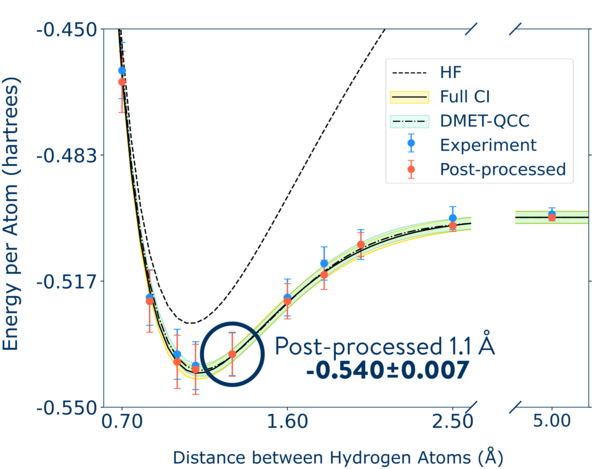
The system studied in this notebook is characterized by a distance of 1.1\(\overset{\circ}{A}\) between hydrogen atoms, and is built in the MINAO basis. The emphasis on this pipeline is to retrieve electronic correlation energy while leveraging the power of NISQ devices. A full potential energy curve has been computed in [Kawashima et al., 2021] to study the repulsive, equilibrium, attractive and dissociative regimes. 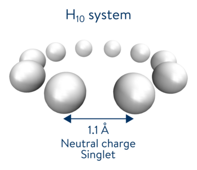
Representing the input molecular data
First, we need to represent the molecular system of interest. Currently, Tangelo accepts some xyz input that specifies individual atoms paired with their corresponding xyz cartesian coordinates. We can pass this information as nested lists containing the atom string and the coordinate tuple (see example below) or as a single string, specifying one atom per line and separating each coordinate with a space.
The openbabel python package can be used to derive the cartesian coordinates from formats such as mol, mol2, ginp, com, pdb (…), and thus provides us with the ability to support your favorite format in the future, maybe even with your contribution to the codebase.
Currently, this package works with molecular Hamiltonians represented in second-quantization, which is the formalism almost all proof-of-concept demonstrations of quantum chemistry simulations on quantum hardware have utilized so far. We provide all the necessary functionalities to obtain SecondQuantizedMolecule data and Hamiltonians in order to represent this system adequately from the xyz coordinates. The minimal input for the creation of this object is a nested list of atomic coordinates (a multi-line string can also be thrown at the SecondQuantizedMolecule class).
This object instantiation includes the computation of the mean-field solutions, provided by a Hartree-Fock (HF) calculation. This is the starting point of post-HF calculations that introduce electronic correlation. Besides general molecular information, the SecondQuantizedMolecule contains data about molecular orbitals and spin-orbitals. One well-known use case for this is to freeze molecular orbitals with the frozen_orbitals argument, in order to reduce problem size, for example.
from tangelo import SecondQuantizedMolecule

xyz = [
    ['H', (0.0, 1.780, 0.0)],
    ['H', (-1.046, 1.44, 0.0)],
    ['H', (-1.693, 0.55, 0.0)],
    ['H', (-1.693, -0.55, 0.0)],
    ['H', (-1.046, -1.44, 0.0)],
    ['H', (0.0, -1.78, 0.0)],
    ['H', (1.046, -1.44, 0.0)],
    ['H', (1.693, -0.55, 0.0)],
    ['H', (1.693, 0.55, 0.0)],
    ['H', (1.046, 1.44, 0.0)]
]

mol = SecondQuantizedMolecule(xyz, q=0, spin=0, basis="minao", frozen_orbitals=None)
pprint(mol.__dict__)
{'active_occupied': [0, 1, 2, 3, 4],
'active_virtual': [5, 6, 7, 8, 9],
'basis': 'minao',
'ecp': {},
'frozen_occupied': [],
'frozen_orbitals': None,
'frozen_virtual': [],
'mean_field': RHF object of <class 'pyscf.scf.hf.RHF'>,
'mf_energy': -5.2772722844168225,
'mo_energies': array([-0.71250664, -0.63494046, -0.63486503, -0.4162918 , -0.41611742,
0.07821244, 0.07835203, 0.50868475, 0.50889667, 0.75894782]),
'mo_occ': array([2., 2., 2., 2., 2., 0., 0., 0., 0., 0.]),
'mo_symm_ids': None,
'mo_symm_labels': None,
'n_atoms': 10,
'n_electrons': 10,
'n_mos': 10,
'n_sos': 20,
'q': 0,
'spin': 0,
'symmetry': False,
'uhf': False,
'xyz': [('H', (0.0, 1.78, 0.0)),
('H', (-1.046, 1.44, 0.0)),
('H', (-1.6929999999999996, 0.55, 0.0)),
('H', (-1.6929999999999996, -0.55, 0.0)),
('H', (-1.046, -1.44, 0.0)),
('H', (0.0, -1.78, 0.0)),
('H', (1.046, -1.44, 0.0)),
('H', (1.6929999999999996, -0.55, 0.0)),
('H', (1.6929999999999996, 0.55, 0.0)),
('H', (1.046, 1.44, 0.0))]}Calculating reference energy with classical solvers
For convenience, we provide access to several well-known classical solvers, such as FCI or CCSD. They may be helpful in investigating hybrid approaches pairing both classical and quantum solvers, or obtaining reference numerical results. The latter help us quantify the accuracy of the approaches we investigate in the rest of this notebook.
We find that our use case turns out to be a simple problem for FCI and CCSD, which can both be used in a straightforward way, by passing the molecule at instantiation and then calling the simulate method.
from tangelo.algorithms import FCISolver, CCSDSolver

fci_energy = FCISolver(mol).simulate()
print(f"FCI energy: {fci_energy:.5f}")

ccsd_energy = CCSDSolver(mol).simulate()
print(f"CCSD energy: {ccsd_energy:.5f}")
FCI energy: -5.41008
CCSD energy: -5.40627Exploring approaches using resource estimation and problem decomposition
Now that we have the reference energy, we can try to tackle the same problem with a quantum computer. In order to do that we have to choose an appropriate quantum algorithm that is able to calculate the ground state energy of a molecule. In this tutorial we choose the VQE algorithm. Note that all the other steps in this pipeline are compatible with other quantum algorithms that can be used for the same purpose (like the phase estimation algorithm). VQE is a popular algorithm, and due to it producing very shallow circuits, it is often the choice for proof of concept demonstrations on near-term quantum hardware. See our VQE notebook for more details about this algorithm. Each quantum algorithm has requirements, i.e. its own unique building blocks and parameters. One important parameter to choose when working with VQE is the choice of strategy to build the parametric wave function (ansatz). At the beginning, we use the vanilla version of a well-known ansatze inspired by the Unitary Coupled Cluster operators in chemistry (a.k.a the UCC ansatze).
With this set up in mind, we can leverage Tangelo to estimate the resources required and the cost of this experiment. Later in the document, we show how by leveraging Tangelo and choosing smarter strategies to build an ansazte, one could turn a seemingly intractable problem into one easy to simulate on a quantum hardware. Resource estimation helps us assert the feasibility of an approach with regards to device capabilities (simulator or QPU), or compare it to alternatives, including what is considered state-of-the-art.
Resource estimation is important, as quantum computing is still a nascent field and the current quantum computers have modest capabilities (limited amount of qubits, low gate fidelity, coherence time, etc. It can be one of the drivers of our exploration, and help us identify the most appropriate approaches in our experiments, as well as their bottlenecks, where impactful breakthroughs could make a difference.
Let’s see what happens when we attempt to tackle our use case with the well-known “standard” VQE algorithm, paired with the UCCSD ansatz and using the Jordan-Wigner (JW) qubit mapping:
from tangelo.algorithms.variational import BuiltInAnsatze, VQESolver

# VQE-UCCSD heads-on approach.
vqe_options = {"molecule": mol, "ansatz": BuiltInAnsatze.UCCSD, "qubit_mapping": "jw"}
vqe_solver = VQESolver(vqe_options)
vqe_solver.build()
print(f"\nVQE-UCCSD JW\n{pp.pformat(vqe_solver.get_resources())}\n")
VQE-UCCSD JW
{'circuit_2qubit_gates': 29184,
 'circuit_depth': 32654,
 'circuit_var_gates': 1804,
 'circuit_width': 20,
 'qubit_hamiltonian_terms': 3591,
 'vqe_variational_parameters': 350}
Resource requirements show here a quantum circuit that is way beyond the capabilities of current quantum hardware. Although some devices may easily accommodate 20 qubits, the limited coherence time will cause a circuit like this to return nothing but noise. Therefore, even if these many qubits are accessible, executing such a deep circuit would result in the accumulation of noise and would yield irrelevant numerical results.
Even worse: emulating such a quantum circuit is already a compute-intensive challenge for our classical computers, and can be time-consuming for even top-notch noiseless classical simulators the community has built so far. The numbers of parameters to optimize would require running this circuit many times over, and the size of that space makes converging to accurate results a daunting task in the first place, if not impossible in practice.
Problem decomposition to reduce resource requirements
Problem decomposition is an approach that can be investigated in order to reduce resource requirements, attempting to find the solution to the initial problem by solving a collection of smaller subproblems. This packages offers several problem decomposition techniques, such as DMET, which is the one we explore here (see DMET and ONIOM notebooks for more details).
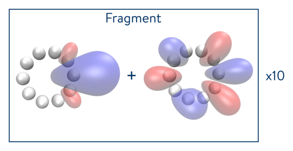
We decompose more and more aggressively to show the impact on resource requirements, going down to fragments of size one atom. Since all fragments play a identical role in our case, for symmetry reasons, we only focus on one of them and treat the others with CCSD to simplify output and calculations.
The get_resources method allows us to peek at some metrics characterizing the fragment circuit, to get a sense of its complexity. What we see is the initial circuit for that particular fragment in our problem instance; we have not yet simulated anything, we merely built the initial objects required for the algorithm.
from tangelo.problem_decomposition import DMETProblemDecomposition
from tangelo.problem_decomposition.dmet import Localization

# DMET-VQE, 5 fragments of size 2 atoms each
dmet_options = {"molecule": mol, "verbose": False,
                "fragment_atoms": [2]*5, "fragment_solvers": ["vqe"] + ["ccsd"]*4,
                "solvers_options": [{"qubit_mapping": "scBK", "initial_var_params": "ones",
                                     "up_then_down": True, "verbose": False}] + [{}]*4}
dmet_solver = DMETProblemDecomposition(dmet_options)
dmet_solver.build()
print(f"DMET-VQE-UCCSD, 5 fragments \n{pp.pformat(dmet_solver.get_resources()[0])}\n")

# DMET-VQE, 10 fragments of size 1 atom each
dmet_options = {"molecule": mol, "verbose": False,
                "fragment_atoms": [1]*10, "fragment_solvers": ["vqe"] + ["ccsd"]*9,
                "solvers_options": [{"qubit_mapping": "scBK", "initial_var_params": "ones",
                                     "up_then_down": True, "verbose": False}] + [{}]*9}
dmet_solver = DMETProblemDecomposition(dmet_options)
dmet_solver.build()
print(f"DMET-VQE-UCCSD, 10 fragments \n{pp.pformat(dmet_solver.get_resources()[0])}\n")
DMET-VQE-UCCSD, 5 fragments
{'circuit_2qubit_gates': 1072,
'circuit_depth': 1461,
'circuit_var_gates': 144,
'circuit_width': 6,
'qubit_hamiltonian_terms': 325,
'vqe_variational_parameters': 14}
DMET-VQE-UCCSD, 10 fragments
{'circuit_2qubit_gates': 4, 'circuit_depth': 14, 'circuit_var_gates': 4, 'circuit_width': 2, 'qubit_hamiltonian_terms': 9, 'vqe_variational_parameters': 2}
The next calculation will be carried out with ten fragments of one atom (one fragment and bath orbitals), as depicted in the figure below.
Validating the desired approach with simulators
The idea behind DMET is to decompose a molecular system into its constituent fragments and its environment. Each fragment is treated independently and recombined at the end to recover the full molecular energy. DMET is an iterative process: at each iteration, the chemical potential is used to adjust both the total number of electrons in the system and in the fragment Hamiltonian. Through the adjustment of the chemical potential, we iterate until the number of electrons in all of the fragments, taken together, becomes equal to the total number of electrons in the entire system, within a user-defined threshold.
The algorithm then stops and the electronic structure is returned. For more information, see the DMET notebook on the subject.
Aggressively decomposing this system into 10 fragments of size 1 atom returns resource requirements that seem much more tractable for existing quantum devices, and seem appealing. But we know nothing about the accuracy we can expect from this approach, which relies on VQE to solve our subproblems. The fragments yield quantum circuits of a size that is very manageable for classical simulators, which can support us in the next steps.
Classical simulation of a quantum circuit
Quantum computers currently have limited access and capability. To study the applications of quantum computing on problem instances of reasonable size, we can use classical simulators and emulators in order to anticipate the behavior of quantum algorithms on real devices, in the presence or absence of noise.
This package provides a submodule called linq, which supports a collection of open-source quantum circuit simulators delivering different performance and features. We are free to choose the most relevant backend for our use cases, thinking about resource requirements, use of shots, presence or absence of noise, and accuracy of simulation, for example. Our algorithms manipulate circuits in our own intermediary representation, and a variety of functions exist in order to convert these objects into popular formats, compatible with other open-source tools.
The simulate method below runs the DMET algorithm using a simulator backend. We could specify the desired backend in the variable dmet_options described above when creating the DMETProblemDecomposition object. We however did not, and the current default choice is to go for a noiseless simulator: since our package relies on openfermion, which installs cirq as a dependency, cirq will be the default backend unless qulacs is found in your environment. Currently other supported local backends include qiskit and QDK.
dmet_energy = dmet_solver.simulate()print(f" DMET-VQE 10 fragments: {dmet_energy:.5f}\n Difference with FCI: {abs(dmet_energy-fci_energy):E}") DMET-VQE 10 fragments: -5.40161
Difference with FCI: 8.464849E-03Minimizing the amount of resources needed for the hardware experiment
Both DMET and VQE are iterative methods: running all the quantum circuits arising in this algorithm with high accuracy on a quantum device would require a number of measurements and runtime beyond what is reasonable on the few quantum processors available today. A more reasonable experiment in the meantime may consist of looking at a single step, and reflect on whether or not this suggests that with more time and resources we could successfully run the whole algorithm on a quantum device, in theory.
In the following section, we decide to have a look at the very last step of the DMET-VQE process, for a single fragment: it resulted in a quantum circuit obtained through classical optimization, which can be used to compute the total energy of the system. Because of the symmetry in our use case, the total energy can be calculated by multiplying the fragment energy by the number of fragments. Thanks to the previous section, we know that we can be critical of these results and compare them to the ones obtained with DMET-VQE with a noiseless simulator, or even the FCI results.
The quantum_fragments_data attribute of our DMET solver object allows us to retrieve fragment information for those who were mapped to a quantum solver. In the case of VQE, this allows us to access the qubit Hamiltonian and quantum circuit obtained after running simulate.
# Retrieving the DMET fragment information computed with VQE.
fragment, fragment_qb_ham, fragment_circuit = dmet_solver.quantum_fragments_data[0]

print(fragment_circuit)
Circuit object. Size 22
X target : [0]
X target : [1]
RX target : [0] parameter : 1.5707963267948966
RZ target : [0] parameter : 3.1415958073076995 (variational)
RX target : [0] parameter : -1.5707963267948966
RX target : [1] parameter : 1.5707963267948966
RZ target : [1] parameter : 3.1415958073076995 (variational)
RX target : [1] parameter : -1.5707963267948966
RX target : [0] parameter : 1.5707963267948966
H target : [1]
CNOT target : [1] control : [0]
RZ target : [1] parameter : 1.658627529909104 (variational)
CNOT target : [1] control : [0]
H target : [1]
RX target : [0] parameter : -1.5707963267948966
H target : [0]
RX target : [1] parameter : 1.5707963267948966
CNOT target : [1] control : [0]
RZ target : [1] parameter : 1.658627529909104 (variational)
CNOT target : [1] control : [0]
RX target : [1] parameter : -1.5707963267948966
H target : [0]
Minimizing the number of measurements needed
The computation of the total energy with DMET requires us to compute the 1- and 2-electron Reduced Density Matrices (1- and 2-RDM). Computing the entries of these matrices requires us to have a look at each term present in the fermionic Hamiltonian of our fragment, apply the same qubit mapping as used in the rest of the DMET algorithm, and compute the expectation value of the resulting qubit operator with regards to our fragment_circuit.
It turns out that different entries sometimes require running the fragment_circuit and measuring the qubits in the same computational bases. Since the DMET energy of a molecular system is a real number, it also means that qubit terms with imaginary coefficients are not relevant. Using this information, we scan the RDMs to find what terms/computational bases actually contribute to the calculation, in order to minimize computation.
Instead of returning them as a list, we agglomerate these terms into a QubitOperator object (a subclass of Openfermion’s QubitOperator), which also keeps track of their prefactor.
from tangelo.toolboxes.operators import FermionOperator, QubitOperator
from tangelo.toolboxes.qubit_mappings.mapping_transform import fermion_to_qubit_mapping

# Find all the measurement bases that are needed to compute the RDMs.
# Accumulate them in a QubitOperator object to manipulate them afterwards.
qubit_op_rdm = QubitOperator()
bases_to_measure = set()

for term in fragment.fermionic_hamiltonian.terms:

    # Fermionic term with a prefactor of 1.0.
    fermionic_term = FermionOperator(term, 1.0)

    qubit_term = fermion_to_qubit_mapping(fermion_operator=fermionic_term, mapping="scBK",
                                          n_spinorbitals=fragment.n_active_sos,
                                          n_electrons=fragment.n_active_electrons,
                                          up_then_down=True)
    qubit_term.compress()

    # Loop to go through all qubit terms. Keep new non-empty ones, with non-imaginary coefficient
    for basis, coeff in qubit_term.terms.items():
        if coeff.real != 0 and basis:
            bases_to_measure.add(basis)
            qubit_op_rdm.terms[basis] = coeff

pprint(qubit_op_rdm)
0.25 [X0] +
0.25 [X0 X1] +
0.25 [X0 Z1] +
-0.25 [Y0 Y1] +
0.25 [Z0] +
0.25 [Z0 X1] +
0.25 [Z0 Z1] +
0.25 [X1] +
0.25 [Z1]At first glance, 9 computational bases seem necessary, one per qubit term. However we notice that sometimes a single computational basis can be used to compute the expectation value of several of these qubit terms. For instance, the basis required for Z0Z1 could also be used for Z0 and Z1.
Identifying these computational bases and mapping them to these qubit operators is equivalent to “grouping” Hamiltonian terms, and allows us to narrow it down further. This is not a trivial problem in general, and several algorithms exist in order to attempt this. Groups are not unique, some may be better than others for different reasons (accuracy, or reducing the number of measurements), and the scaling of these algorithms is of utmost importance on more ambitious problem instances.
One of them relies on qubit-wise commutativity, and is shown below. If you would like to know more about this topic, you can have a look at the following references [McClean, J. et al. 2016 and Kandala, A. et al. 2017].
from tangelo.toolboxes.measurements import group_qwc

qwc_map = group_qwc(qubit_op_rdm, seed=0)
print(f"Only execute {len(qwc_map)} circuits, instead of {len(qubit_op_rdm.terms)}.\n")
pprint(qwc_map)
Only execute 5 circuits, instead of 9.
{((0, 'X'), (1, 'X')): 0.25 [X0 X1],
((0, 'X'), (1, 'Z')): 0.25 [X0] +
0.25 [X0 Z1] +
0.25 [Z1],
((0, 'Y'), (1, 'Y')): -0.25 [Y0 Y1],
((0, 'Z'), (1, 'X')): 0.25 [Z0] +
0.25 [Z0 X1] +
0.25 [X1],
((0, 'Z'), (1, 'Z')): 0.25 [Z0 Z1]}Each of the measurement bases here allows us to compute the expectation values of all of the terms it’s mapped to, by running a single quantum circuit. We only need to run 5 circuits on a quantum computer in order to compute everything we need. Let’s put them together quickly: each measurement basis simply adds a few extra “change-of-basis gates”, one per qubit at most, at the end of our fragment quantum circuit.
from tangelo.linq import Circuit, Gate
from tangelo.linq.helpers.circuits.measurement_basis import measurement_basis_gates

# Creation of XX, XZ, ZX, ZZ and YY circuits.
# This is done by appending relevant gates to the quantum circuit representing the quantum state.
quantum_circuit = dict()
for basis in bases_to_measure:
    quantum_circuit[basis] = fragment_circuit + Circuit(measurement_basis_gates(basis))

print(quantum_circuit[((0, "Y"), (1, "Y"))])
Circuit object. Size 24
X target : [0]
X target : [1]
RX target : [0] parameter : 1.5707963267948966
RZ target : [0] parameter : 3.1415958073076995 (variational)
RX target : [0] parameter : -1.5707963267948966
RX target : [1] parameter : 1.5707963267948966
RZ target : [1] parameter : 3.1415958073076995 (variational)
RX target : [1] parameter : -1.5707963267948966
RX target : [0] parameter : 1.5707963267948966
H target : [1]
CNOT target : [1] control : [0]
RZ target : [1] parameter : 1.658627529909104 (variational)
CNOT target : [1] control : [0]
H target : [1]
RX target : [0] parameter : -1.5707963267948966
H target : [0]
RX target : [1] parameter : 1.5707963267948966
CNOT target : [1] control : [0]
RZ target : [1] parameter : 1.658627529909104 (variational)
CNOT target : [1] control : [0]
RX target : [1] parameter : -1.5707963267948966
H target : [0]
RX target : [0] parameter : 1.5707963267948966
RX target : [1] parameter : 1.5707963267948966
Picking the number of measurements
The more shots (measurements) we take, the more accurate the depiction of our prepared quantum state, which is then used to compute expectation values. On one hand, we would like to take as many as possible for the sake of accuracy. On the other hand, the number of shots is directly related to cost in time and resources of our experiment, which we need to keep within the acceptable budget for the experiment.
It makes sense for expectation values of terms with larger coefficients to be computed with higher accuracy (i.e more shots), as the coefficient may amplify any error committed by the quantum computer during its approximation. Conversely, terms with coefficients that are close to zero may individually contribute less, or even not matter, depending on the desired accuracy of the final results. If the expectation values of several qubit terms can be computed using a single computational basis, it would then make sense to pick the number of shots by looking at the one with the biggest coefficient.
The community is actively researching ways to provide good estimates, from simple heuristics to more advanced approaches that take into account the problem’s specifics and underlying principles. We look forward to supporting more of them in this package, hopefully with your help!
Below, we show you what the numbers would be for a simple heuristic stating that “when we multiply the number of shots by 100, we gain an extra digit of accuracy”, coming from binomial sampling. We use that heuristic on each of our 5 measurement bases, requesting 2 digits of accuracy. In our case, since all qubit terms have a coefficient with absolute value of 0.25, the number of measurements this method returns is identical for all 5 circuits.
from tangelo.toolboxes.measurements.estimate_measurements import get_measurement_estimate

measurements = {k: get_measurement_estimate(v, digits=2) for k,v in qwc_map.items()}
pprint(measurements)
{((0, 'X'), (1, 'X')): {((0, 'X'), (1, 'X')): 62500},
((0, 'X'), (1, 'Z')): {((0, 'X'),): 62500,
((0, 'X'), (1, 'Z')): 62500,
((1, 'Z'),): 62500},
((0, 'Y'), (1, 'Y')): {((0, 'Y'), (1, 'Y')): 62500},
((0, 'Z'), (1, 'X')): {((0, 'Z'),): 62500,
((0, 'Z'), (1, 'X')): 62500,
((1, 'X'),): 62500},
((0, 'Z'), (1, 'Z')): {((0, 'Z'), (1, 'Z')): 62500}}We decided to go with 10,000 shots per circuit, as we deemed it to be within acceptable accuracy and mesurement budget constraints. This further emphasizes the need to come up with approaches that reduce the number of measurements needed, and algorithms that can make the most of each measurement, in terms of information and accuracy.
n_shots = 10000Circuit compilation and optimization
The gate set we use to express our circuits so far contains widely-used generic gates such as H, CNOT and RX, RY, RZ gates. But these are not necessarily part of the native gate set supported by the quantum device this circuit will run on. That is, our circuits must be first expressed in an equivalent sequence of native gates supported by the device. Furthermore, applying gate identities to these circuits may yield simpler equivalent ones requiring a lower amount of gates (or even qubits), which may lead to better accuracy.
This overall process of compilation to a native gate set and further optimization of the circuit is challenging, and is usually handled by hardware manufacturers at runtime. Some document and expose these low-level functionalities through their API. In addition to that, there are several open-source projects that specifically target the issue of compilation and circuit optimization for diverse architectures or gate sets: we look towards supporting some of them in the future.
Submitting an experiment to a quantum device
This package offers several ways to submit experiments on quantum devices. Below, a few examples of how it is possible to do so through quantum cloud services, and converting your circuit in the relevant formats.
Using QEMIST Cloud
The simplest way to submit an experiment to any device available in the supported quantum cloud services is through QEMIST Cloud’s client library, allowing users to run quantum hardware experiments using their QEMIST Cloud account credentials and credits. This is possible if you have access to QEMIST Cloud, and have installed qemist-client Python package. For more details about this feature, please don’t hesitate to refer to our dedicated notebook, and reach out to us about QEMIST Cloud.
Below, a simple code snippet illustrating how to run 10,000 shots of the YY circuit on IonQ’s hardware, through Amazon’s Braket quantum cloud services:
# Retrieve both these values from your QEMIST Cloud dashboard
import os
os.environ['QEMIST_PROJECT_ID'] = "your_project_id_string"
os.environ['QEMIST_AUTH_TOKEN'] = "your_qemist_authentication_token"

# Estimate, submit and get the results of your job / quantum task through our wrappers
from tangelo.linq.qpu_connection import QEMISTCloudConnection

qcloud_connection = QEMISTCloudConnection()
circuit_YY = quantum_circuit[((0, "Y"), (1, "Y"))]price_estimates = qcloud_connection.job_estimate(circuit_YY, n_shots=n_shots)
print(price_estimates)
backend = 'arn:aws:braket:::device/qpu/ionq/ionQdevice'
# This two commands would respecfully submit the job to the quantum device and make a blocking call
# to retrieve the results, through a job ID returned by QEMIST Cloud
job_id = qcloud_connection.job_submit(circuit_YY, n_shots=n_shots, backend=backend)
freqs, raw_data = qcloud_connection.job_results(job_id)Output:
{'arn:aws:braket:::device/qpu/ionq/ionQdevice': 100.3, 'arn:aws:braket:::device/quantum-simulator/amazon/sv1': 3.8, 'arn:aws:braket:us-west-1::device/qpu/rigetti/Aspen-M-1': 3.8}Using a cloud API and format conversion
The utility functions in tangelo.linq allow us to convert our generic Circuit objects into a variety of formats supported by other open-source packages and services, such as Amazon’s Braket and Microsoft’s Azure Quantum.
You can thus convert a Circuit object into the desired format and use the API of those services directly in order to reach a QPU or an online simulator if you wish to do so. The example below shows how to convert a Circuit object into the Braket format. Provided that you have a Braket account, the submission process is pretty straightforward, as demonstrated by the documentation
from tangelo.linq.translator import translate_circuit

braket_circuit = translate_circuit(circuit_YY, target="braket")
print(braket_circuit)
T : |0| 1 | 2 | 3 | 4 |5| 6 |7| 8 | 9 |10| 11 |12| 13 | 14 |
q0 : -X-Rx(1.57)-Rz(3.14)-Rx(-1.57)-Rx(1.57)-C----------C-Rx(-1.57)-H--------C-----------C--H---------Rx(1.57)-
| | | |
q1 : -X-Rx(1.57)-Rz(3.14)-Rx(-1.57)-H--------X-Rz(1.66)-X-H---------Rx(1.57)-X--Rz(1.66)-X--Rx(-1.57)-Rx(1.57)-
T : |0| 1 | 2 | 3 | 4 |5| 6 |7| 8 | 9 |10| 11 |12| 13 | 14 |Likewise, Azure Quantum supports a number of formats. Our package provides similar “translation” functions allowing us to produce a Circuit object into a Q#, qiskit or a cirq format, for example (see cell below) . Provided we have a working Azure Quantum environment, our circuits can be submitted using their API as detailed in the previous link.
from tangelo.linq.translator import translate_circuit

cirq_circuit = translate_circuit(circuit_YY, target="cirq")
print(cirq_circuit)
0: ───I───X───Rx(0.5π)───Rz(π)───Rx(-0.5π)───Rx(0.5π)───@────────────────@───Rx(-0.5π)───H──────────@────────────────@───H───────────Rx(0.5π)───
│ │ │ │
1: ───I───X───Rx(0.5π)───Rz(π)───Rx(-0.5π)───H──────────X───Rz(0.528π)───X───H───────────Rx(0.5π)───X───Rz(0.528π)───X───Rx(-0.5π)───Rx(0.5π)───Emulation on a noisy backend
Since many open-source packages support noisy simulation and hardware providers put out some information about their devices, you could be interested in performing the noisy simulation of your quantum circuits. In particular, this could help you get an idea of the performance of your algorithm on a target device or get a sense of the performance a device would require for your algorithm to return an answer within the desired accuracy, without requiring access to a QPU.
We provide a general interface giving you access to several simulator backends in order to facilitate the simulation of such circuits. You are free to use the “translate” functions of tangelo in order to use the API provided by your favorite open-source package directly if you’d like, as this offers finer control and maybe more features.
Below, an example using our generic NoiseModel object and specifying the backend when calling simulate. Here we show an example applying a depolarization channel to specific gates, each with a given probability.
from tangelo.linq import get_backend
from tangelo.linq.noisy_simulation import NoiseModel

nmp = NoiseModel()
nmp.add_quantum_error("CNOT", "depol", 0.01)
nmp.add_quantum_error("RZ", "depol", 0.005)
nmp.add_quantum_error("H", "depol", 0.005)

backend = get_backend(target="cirq", n_shots=n_shots, noise_model=nmp)
# Getting frequencies for each circuits.
freq_dict = dict()
for term, circuit in quantum_circuit.items():
freq_dict[term], _ = backend.simulate(circuit)
pp.pprint(freq_dict[((0, "Y"), (1, "Y"))]){'00': 0.3003, '01': 0.2004, '10': 0.2071, '11': 0.2922}Post-processing
In our publication, we used the DMET-VQE approach paired with the Qubit Coupled-Cluster (QCC) ansatz, in order to generate our fragment circuits. Although IonQ have their own automated tools to perform quantum circuit compilation and optimization for their device, they had a very close look with us at these circuits, in an attempt to help the quantum device get results as accurate as possible. For further details, you can have a look at figure 1c in our publication.
In particular, the compilation and optimization process in that native gate set allowed us to realize that the circuits corresponding to the XZ and ZX bases were identical, up to a reordering of the qubits. This meant that only one of these two circuits was really necessary to run on the device, in order to derive the frequencies for both bases. This anecdote reinforces the need for our community to develop tools to facilitate gaining such insights, as part of larger workflows and more complex problems.
For the purpose of our experiments, we thus executed 4 circuits with 10,000 shots each on the device. Using the results, we derived all other quantities relevant to us. In order to reproduce the results studied in our article, we use in the following the values that were obtained from running the circuits run on the device. We use these values to compute one of the data-points presented in our work.
# DMET-QCC experimental frequencies.
freq_dict = {((0, "Z"), (1, "Z")): {"00": 0.0093, "10": 0.0000, "01": 0.0000, "11": 0.9907},
             ((0, "X"), (1, "Z")): {"00": 0.0047, "10": 0.0047, "01": 0.4959, "11": 0.4947},
             ((0, "X"), (1, "X")): {"00": 0.2059, "10": 0.2940, "01": 0.2947, "11": 0.2054},
             ((0, "Y"), (1, "Y")): {"00": 0.2854, "10": 0.2114, "01": 0.2017, "11": 0.3015}}
# Derived thanks to observations after compilation and optimization: similar to XZ
freq_dict[((0, "Z"), (1, "X"))] = {"00": 0.0047, "10": 0.4959, "01": 0.0047, "11": 0.4947}We can then compute the expectation values of the different qubit operators of interest by using these frequencies. For simplicity, we manually compute all 9 of them, from the 5 histograms. Note that because the term grouping based on qubit-wise commutativity is not unique, several of these circuits could be used to compute the output of a different computational basis: in our case, it means that we overall have 20,000 shots worth of data by aggregating the two relevant histograms for certain entries,
We provide a Histogram helper class and the aggregate_histogram function to facilitate this kind of operation. This data-structure encapsulates the dictionary of frequencies and the number of shots used to build it, which is used as a "weight" when aggregating with other histograms. If we keep track of the number of shots used for each computational basis (with a dictionary for example) then it is pretty straightforward to leverage that helper class. In our case it is even easier: all jobs used the name number of shots.
from tangelo.toolboxes.post_processing import Histogram, aggregate_histograms

# Turn dictionary of frequencies into Histogram objects
freq_hists = {k: Histogram(freqs, n_shots) for k, freqs in freq_dict.items()}

# Compute the other Histogram objects by aggregating the ones obtained in the experiment
freq_hists[((0, 'Z'),)] = aggregate_histograms(freq_hists[((0, 'Z'), (1, 'Z'))], freq_hists[((0, 'Z'), (1, 'X'))])
freq_hists[((1, 'Z'),)] = aggregate_histograms(freq_hists[((0, 'Z'), (1, 'Z'))], freq_hists[((0, 'X'), (1, 'Z'))])
freq_hists[((0, 'X'),)] = aggregate_histograms(freq_hists[((0, 'X'), (1, 'Z'))], freq_hists[((0, 'X'), (1, 'X'))])
freq_hists[((1, 'X'),)] = aggregate_histograms(freq_hists[((0, 'Z'), (1, 'X'))], freq_hists[((0, 'X'), (1, 'X'))])

expectation_values = {term: hist.get_expectation_value(term) for term, hist in freq_hists.items()}
pprint(expectation_values)
{((0, 'X'),): 0.0011999999999999789,
((0, 'X'), (1, 'X')): -0.17740000000000003,
((0, 'X'), (1, 'Z')): -0.0012000000000000344,
((0, 'Y'), (1, 'Y')): 0.17379999999999998,
((0, 'Z'),): -0.9813000000000001,
((0, 'Z'), (1, 'X')): -0.0012000000000000344,
((0, 'Z'), (1, 'Z')): 1.0,
((1, 'X'),): 0.0005000000000001115,
((1, 'Z'),): -0.9813000000000001}For a more systematic approach on larger problem instances, it would however be better to reuse the map used for grouping qubit terms earlier, and “reverse” it: that is, associate each desired basis with the set of bases for which a circuit was actually run. Assuming we kept track of shots for each circuit, we could then use a function to compute all entries of freq_dict as weighted average of the frequencies obtained from the device.
From the expectation values, we can then compute the one- and two-electron reduced density matrices:
import numpy as np
import itertools

def compute_rdms(fragment, expectation_values):
    onerdm = np.zeros((fragment.n_active_sos,) * 2, dtype=complex)
    twordm = np.zeros((fragment.n_active_sos,) * 4, dtype=complex)

    for term in fragment.fermionic_hamiltonian.terms:
        length = len(term)

        # Fermionic term with a prefactor of 1.0.
        fermionic_term = FermionOperator(term, 1.0)

        qubit_term = fermion_to_qubit_mapping(fermion_operator=fermionic_term, mapping="scBK",
                                              n_spinorbitals=fragment.n_active_sos,
                                              n_electrons=fragment.n_active_electrons,
                                              up_then_down=True)
        qubit_term.compress()

        # Loop to go through all qubit terms.
        eigenvalue = 0.
        for qubit_term, coeff in qubit_term.terms.items():
            if coeff.real != 0:
                exp_val = expectation_values[qubit_term] if qubit_term else 1.
                eigenvalue += coeff * exp_val

        # Put the values in np arrays (differentiate 1- and 2-RDM)
        if length == 2:
            iele, jele = (int(ele[0]) for ele in tuple(term[0:2]))
            onerdm[iele, jele] += eigenvalue
        elif length == 4:
            iele, jele, kele, lele = (int(ele[0]) for ele in tuple(term[0:4]))
            twordm[iele, lele, jele, kele] += eigenvalue

        onerdm_spinsum = np.zeros((fragment.n_active_mos,)*2, dtype=complex)
        twordm_spinsum = np.zeros((fragment.n_active_mos,)*4, dtype=complex)

        # Construct spin-summed 1-RDM.
        for i, j in itertools.product(range(fragment.n_active_sos), repeat=2):
            onerdm_spinsum[i//2, j//2] += onerdm[i, j]

        # Construct spin-summed 2-RDM.
        for i, j, k, l in itertools.product(range(fragment.n_active_sos), repeat=4):
            twordm_spinsum[i//2, j//2, k//2, l//2] += twordm[i, j, k, l]

    return onerdm, twordm, onerdm_spinsum, twordm_spinsum

onerdm, twordm, onerdm_spinsum, twordm_spinsum = compute_rdms(fragment, expectation_values)
Finally, we compute the fragment energy from the 1- and 2-RDMs:
def compute_electronic_fragment_energy(fragment, onerdm, twordm):
    """Calculate the fragment energy."""

    norb = fragment.t_list[0]
    mo_coeff = fragment.mean_field.mo_coeff
    fock = fragment.fock
    oneint = fragment.one_ele
    twoint = fragment.two_ele

    # Calculate the one- and two- RDMs for DMET energy calculation (Transform to AO basis).
    one_rdm = mo_coeff @ onerdm @ mo_coeff.T

    twordm = np.einsum("pi,ijkl->pjkl", mo_coeff, twordm)
    twordm = np.einsum("qj,pjkl->pqkl", mo_coeff, twordm)
    twordm = np.einsum("rk,pqkl->pqrl", mo_coeff, twordm)
    twordm = np.einsum("sl,pqrl->pqrs", mo_coeff, twordm)

    # Calculate fragment expectation value.
    fragment_energy_one_rdm = 0.25 * np.einsum("ij,ij->", one_rdm[: norb, :], fock[: norb, :] + oneint[: norb, :]) \
        + 0.25 * np.einsum("ij,ij->", one_rdm[:, : norb], fock[:, : norb] + oneint[:, : norb])

    fragment_energy_twordm = 0.125 * np.einsum("ijkl,ijkl->", twordm[: norb, :, :, :], twoint[: norb, :, :, :]) \
        + 0.125 * np.einsum("ijkl,ijkl->", twordm[:, : norb, :, :], twoint[:, : norb, :, :]) \
        + 0.125 * np.einsum("ijkl,ijkl->", twordm[:, :, : norb, :], twoint[:, :, : norb, :]) \
        + 0.125 * np.einsum("ijkl,ijkl->", twordm[:, :, :, : norb], twoint[:, :, :, : norb])

    fragment_energy = fragment_energy_one_rdm + fragment_energy_twordm

    return fragment_energy.real


# Compute fragment energy as core repulsion fragment energy plus electron-correlation energy
core_constant = dmet_solver.orbitals.core_constant_energy / 10
e_fragment = compute_electronic_fragment_energy(fragment, onerdm_spinsum, twordm_spinsum) + core_constant
print(f" DMET-VQE QCC 1 fragment: {e_fragment:.5f}\n Difference with FCI: {abs(e_fragment-(fci_energy/10)):E}")
DMET-VQE QCC 1 fragment: -0.55205
Difference with FCI: 1.104160E-02Error mitigation
The next step in our post-processing is focused on error mitigation. Due to noise, the hardware produces a mixed state, which reduces the accuracy of our observables. The ultimate tool against noise is error correction. However, employing error correction is prohibitively expensive in terms of the quantum resources required and out of reach of near-term quantum hardware (hence the “Noisy” in NISQ). Although error correction is not currently available, we can still utilize clever ideas and leverage the known symmetries of the input problem to post-process the raw results coming form the hardware to mitigate the noise to some extent. Tangelo aims to provide a collection of noise mitigation techniques.
As an error-mitigation strategy in our DMET experiment, we use a density matrix purification technique based on McWeeny’s purification method [Truflandier et al., 2016] to purify our noisy state to the dominant eigenvector. This is an iterative method which imposes the idempotency condition according to:
\[ P^{\text{new}}_{pqrs}=3(P^{\text{old}}_{pqrs})^{2}-2(P^{\text{old}}_{pqrs})^{3}\]
For our particular experiment, we can use this method for the 2-RDM since our fragments consist of two electrons – thus the 2-RDM is the full density matrix, and idempotency can be imposed. In general, applying the technique to 2-RDMs of higher electron systems would require the more sophisticated N-representability conditions [Rubin et al., 2018].
from tangelo.toolboxes.post_processing.mc_weeny_rdm_purification import mcweeny_purify_2rdm

onerdm_spinsum, twordm_spinsum = mcweeny_purify_2rdm(twordm.real, conv=1e-2)
e_pure_fragment = compute_electronic_fragment_energy(fragment, onerdm_spinsum, twordm_spinsum) + core_constant
print(f" DMET-VQE QCC 1 fragment: {e_pure_fragment:.5f}\n Difference with FCI: {abs(e_pure_fragment-(fci_energy/10)):E}")
DMET-VQE QCC 1 fragment: -0.54020
Difference with FCI: 8.035695E-04Statistical analysis of results
Experimental data requires a measure of its uncertainty. As it is often prohibitively expensive to collect large amount of data on quantum computers for the purpose of estimating uncertainty, we generate statistics from our dataset using an established method called bootstrapping [Efron, B. et al., 1994]. For each histogram obtained from our experiment, we resample with replacement from that distribution to generate new histograms of the same sample size. We then use these histograms to calculate a new set of expectation values, RDMs, and total energies. This process is repeated many times, and from those outcomes we calculate the average energy and standard deviation of our experiment.
In our publication, this process was repeated 10,000 times and led to a result of -0.540 ±0.007 Hartree.
# Bootstrap method.
fragment_energies = list()

for n in range(1000): # Was 10000 in our publication

    # Step 1-2: draw random bootstrap sample and construct new histograms.
    resample_freq = {term: hist.resample(n_shots) for term, hist in freq_hists.items()}

    # Step 3-4: compute expectation values.
    expectation_values = {term: hist.get_expectation_value(term) for term, hist in resample_freq.items()}

    # Step 5: construct 1- and 2-RDMs.
    onerdm, twordm, _, _ = compute_rdms(fragment, expectation_values)
    onerdm_spinsum, twordm_spinsum = mcweeny_purify_2rdm(twordm.real, conv=1e-2)

    # Step 6: calculate the total energy.
    e_fragment = compute_electronic_fragment_energy(fragment, onerdm_spinsum, twordm_spinsum) + core_constant
    fragment_energies.append(e_fragment)

    # Step 7: Repeat steps 1-6.

# Step 8: calculate the mean and standard deviation.
mean = np.mean(fragment_energies)
stdev = np.std(fragment_energies, ddof=1)
print(f" Bootstrap DMET-VQE QCC energy {mean:.4f}±{stdev:.4f}.")
Bootstrap DMET-VQE QCC energy -0.5394±0.0059.This is in agreement with the published results [Kawashima et al., 2021], which repeats this overall workflow for various H-H distances and thoroughly analyzes repulsive, equilibrium, attractive and dissociative regimes.
Closing words
This notebook showed how Tangelo can assist us in implementing end-to-end workflows, which can lead to successful hardware experiments and peer-reviewed publications in the field.
On the one hand, it highlights how problem decomposition can make larger molecular systems amenable to NISQ devices, in combination with pre- and post-processing methods aiming at reducing resource requirements or improving accuracy. Such approaches may play an essential role in applying quantum computers to the study of larger, industrially relevant, chemical systems.
On the other hand, it illustrates the complexity of such experiments and the necessity for the community to keep developing tools that can be articulated together to cover elaborate end-to-end workflows. From a molecule, we have built a quantum computing experiment which involved numerous steps, some related to quantum chemistry algorithms, some tackling the challenges of practical experiments on quantum computers.
We look forward to further developing these tools with the help of the community, in order to both take us a step closer to making quantum computing applicable to real-world problems, but also simply to give you the satisfaction of running a successful experiment yourself soon.
References
- Efron, B. & Tibshirani, R. J. An Introduction to the Bootstrap (CRC press, 1994))
- Kassal, I., Whitfield, J. D., Perdomo-Ortiz, A., Yung, M.-H. & Aspuru-Guzik, A. Simulating Chemistry Using Quantum Computers. Annual Review of Physical Chemistry 62, 185–207 (2011).
- Knizia, G. & Chan, G. K. L. Density matrix embedding: A simple alternative to dynamical mean-field theory. Physical Review Letters 109, 186404–186404 (2012).
- Knizia, G. & Chan, G. K. L. Density matrix embedding: A strong-coupling quantum embedding theory. Journal of Chemical Theory and Computation 9, 1428–1432 (2013).
- Peruzzo, A. et al. A variational eigenvalue solver on a quantum processor. Nature Communications 5, 4213–4213 (2013).
- L. A. Truflandier, R. M. Dianzinga, and D. R. Bowler,Generalized canonical purification for density matrixminimization, J. Chem. Phys. 144, 091102 (2016).
- McClean, J., Romero, J., Babbush, R. & Aspuru-Guzik, A.. The theory of variational hybrid quantum-classical algorithms. New J. Phys. 18 023023 (2016).
- McClean, J., Romero, J., Babbush, R. & Aspuru-Guzik, A.. The theory of variational hybrid quantum-classical algorithms. New J. Phys. 18 023023 (2016).
- N. C. Rubin, R. Babbush, and J. McClean, Application of fermionic marginal constraints to hybrid quantum algorithms, New Journal of Physics 20, 053020 (2018).
- Cao, Y. et al. Quantum Chemistry in the Age of Quantum Computing. Chemical Reviews 119, 10856–10915 (2019).
- Y. Nam, J.-S. Chen, N. C. Pisenti, K. Wright, C. Delaney, D. Maslov, K. R. Brown, S. Allen, J. M. Amini, J. Apisdorf, K. M. Beck, A. Blinov, V. Chaplin, M. Chmielewski, C. Collins, S. Debnath, A. M. Ducore, K. M. Hudek, M. Keesan, S. M. Kreikemeier, J. Mizrahi, P. Solomon, M. Williams, J. D. Wong-Campos, C. Monroe, and J. Kim, Ground-state energy estimation of the water molecule on a trapped ion quantum computer, npj Quantum Information 6, 33 (2019).
- Kawashima, Y. et al. Efficient and Accurate Electronic Structure Simulation Demonstrated on a Trapped-Ion Quantum Computer. arXiv:2102.07045 [quant-ph] (2021).
- Bharti, K. et al. Noisy intermediate-scale quantum (NISQ) algorithms. arXiv:2101.08448 [quant-ph] (2021).