# Installation of tangelo if not already installed.
try:
    import tangelo
except ModuleNotFoundError:
    !pip install git+https://github.com/sandbox-quantum/Tangelo.git@develop --quiet
!pip install qulacs pyscf --quietDensity Matrix Embedding Theory (DMET)
This notebook introduces a problem-decomposition technique called DMET (Density-Matrix Embedding Technique), which enables us to break down a molecular systems into a collection of subproblems with lower computational resource requirements.
Such approaches enable us to study how combining classical and quantum algorithms may play a role in the resolution of problems beyond toy models, and even maybe provide a configurable and scalable path forward in the future, towards much more ambitious molecular systems.
This notebook assumes that you already have installed Tangelo in your Python environment, or have updated your Python path so that the imports can be resolved. If not, executing the cell below installs the minimal requirements for this notebook.
Table of contents:
1. Introduction
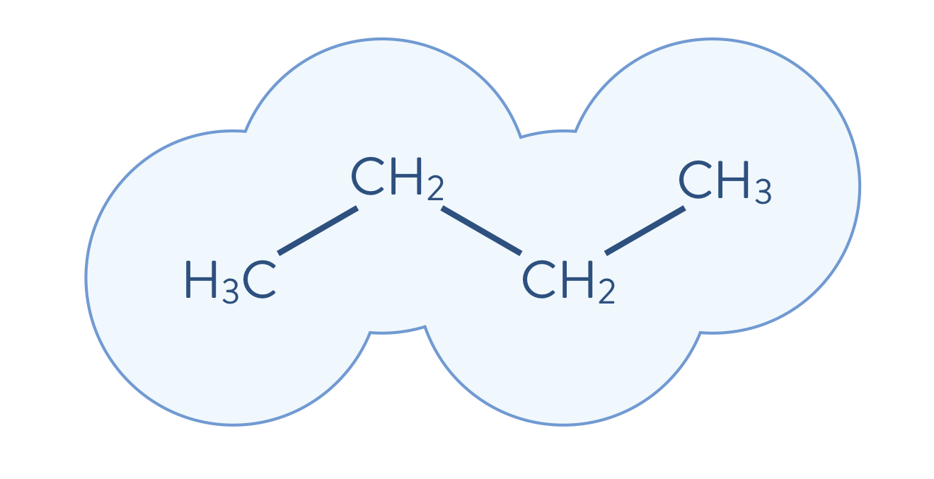
One of the main objectives of quantum chemistry calculations in the area of materials science is to solve the electronic structure problem, \(H\Psi=E\Psi\), as accurately as possible, in order to accelerate the materials design process. In the first example, the butane molecule is shown as an example.
The computational cost for performing accurate calculations of the electronic structure of molecules, however, is usually very expensive. For example, the cost of performing the full CI calculation scales exponentially on a classical computer as the size of the system increases. Therefore, when we target large-sized molecules, those relevant for industry problems, it becomes essential to employ an appropriate strategy for reducing the computational cost. The difficulty is to employ a strategy that consolidate accuracy while reducing computational costs when performing electronic structure calculations. Next, we will developp one of such strategies called Density-Matrix Embedding Theory (DMET).
2. Theory of DMET
The idea is to decompose a molecular system into its constituent fragments and its environment. Each fragment are treated independently and recombined at the end to recover the full molecular energy. This has the advantages of cutting down the maximal computational complexity depending on the biggest fragment and being naturally implemented on parrallel computer. On the other side, the fragmenting comes at the cost of reducing accuraccy of the computation.
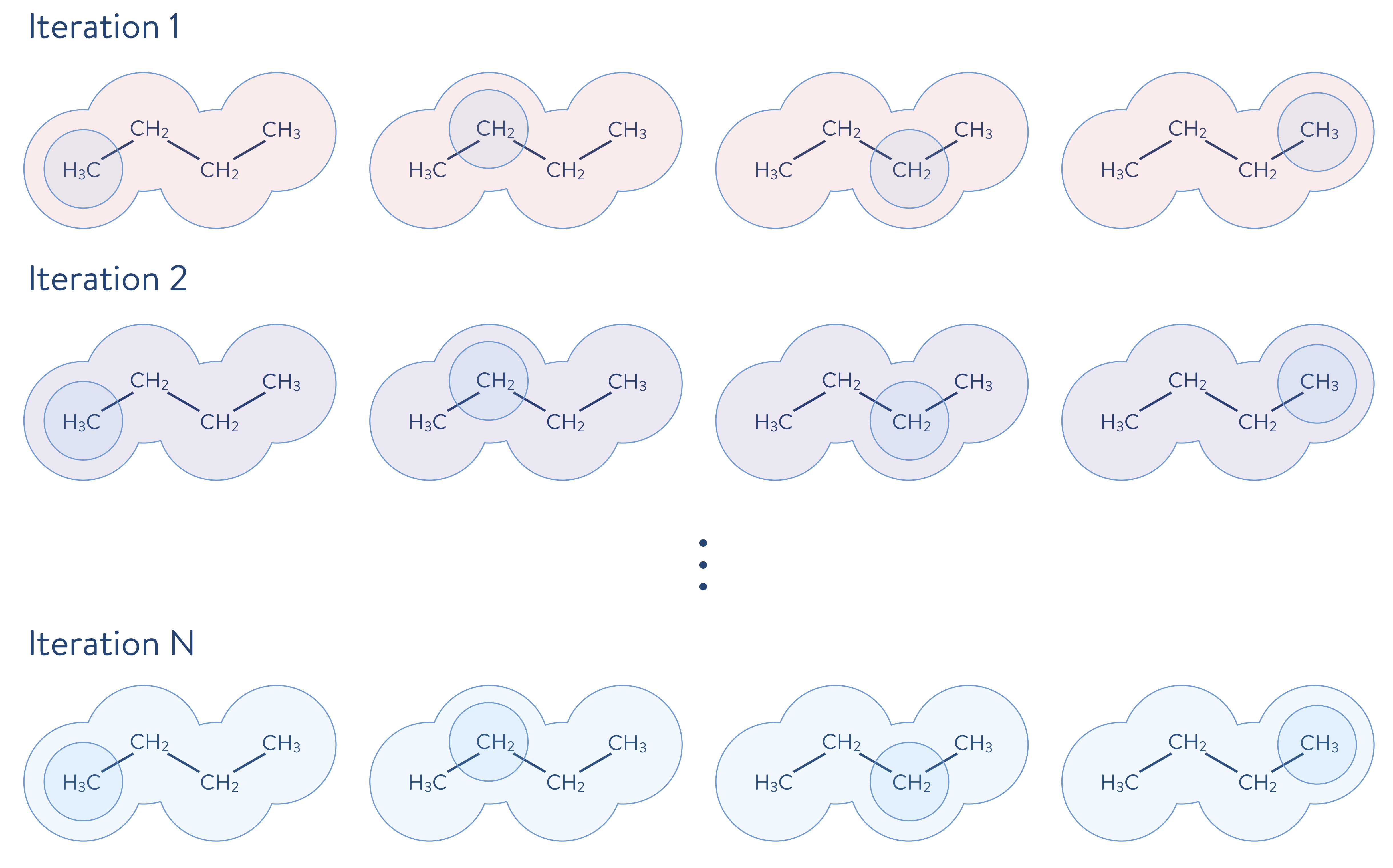
First, the environment is calculated using a less-accurate method than will be used to calculate the electronic structure of a fragment. Then, the electronic structure problem for a given fragment is solved to a high degree of accuracy, which includes the quantum mechanical effects of the environment. The quantum mechanical description is updated (i.e., solved iteratively as shown below) by incorporating the just-performed highly accurate calculation. In the following schematic illustration, the molecule shown above is decomposed into fragments. Each molecular fragment CH\(_\mathrm{3}\) and CH\(_\text{2}\) are the fragments chosen for the electronic structure calculation, with the rest of the molecular system being the surrounding environment.
One successful decomposition approach is the DMET method. The DMET method decomposes a molecule into fragments, and each fragment is treated as an open quantum system that is entangled with each of the other fragments, all taken together to be that fragment’s surrounding environment (or “bath”). In this framework, the electronic structure of a given fragment is obtained by solving the following Hamiltonian, by using a highly accurate quantum chemistry method, such as the full CI method or a coupled-cluster method.
\[ H_{I}=\sum^{\text{frag}+\text{bath}}_{rs} \left[ h_{rs} + \sum_{mn} \left[ (rs|mn) - (rn|ms) \right] D^{\text{(mf)env}}_{mn} \right] a_{r}^{\dagger}a_{s} + \sum_{pqrs}^{\text{frag}+\text{bath}} (pq|rs) a_{p}^{\dagger}a_{r}^{\dagger}a_{s}a_{q} - \mu\sum_{r}^{\text{frag}} a_{r}^{\dagger}a_{r} \]
The expression \(\sum_{mn} \left[ (rs|mn) - (rn|ms) \right] D^{\text{(mf)env}}_{mn}\) describes the quantum mechanical effects of the environment on the fragment, where \(D^{\text{(mf)env}}_{mn}\) is the mean-field electronic density obtained by solving the Hartree–Fock equation. The quantum mechanical effects from the environment are incorporated through the one-particle term of the Hamiltonian. The extra term \(\mu\sum_{r}^{\text{frag}} a_{r}^{\dagger}a_{r}\) ensures, through the adjustment of \(\mu\), that the number of electrons in all of the fragments, taken together, becomes equal to the total number of electrons in the entire system.
3. First example: DMET-CCSD on Butane
Before we proceed, let’s import all the relevant data-structures and classes from tangelo:
# Import for a pretty jupyter notebook.
import json

# Molecule definition.
from tangelo import SecondQuantizedMolecule

# The minimal import for DMET.
from tangelo.problem_decomposition import DMETProblemDecomposition
# Ability to change localization method.
from tangelo.problem_decomposition.dmet import Localization
# Use for VQE ressources estimation vs DMET.
from tangelo.algorithms import VQESolver
# Use for comparison.
from tangelo.algorithms import FCISolver
The first example will show how to partition the system into fragments. A different method for solving electronic structures can be chosen for each fragment, but here we will stick with CCSD. The first thing to do is building the butane molecule object.
butane = """
C   2.142   1.395  -8.932
H   1.604   0.760  -8.260
H   1.745   2.388  -8.880
H   2.043   1.024  -9.930
C   3.631   1.416  -8.537
H   4.169   2.051  -9.210
H   3.731   1.788  -7.539
C   4.203  -0.012  -8.612
H   3.665  -0.647  -7.940
H   4.104  -0.384  -9.610
C   5.691   0.009  -8.218
H   6.088  -0.983  -8.270
H   5.791   0.381  -7.220
H   6.230   0.644  -8.890
"""

# Building the molecule object.
mol_butane = SecondQuantizedMolecule(butane, q=0, spin=0, basis="minao")
The options for the DMET decomposition method are stored in a python dictionary. * molecule: The SecondQuantizedMolecule object. * fragment_atoms: List for the number of atoms in each fragment. Each atoms are chosen with their order in the coordinates definition (variable butane). Also, the sum of all numbers must be equal to total number of atoms in the molecule. * fragment_solvers: A string or a list of string representing the solver for each fragment. The number of items in the list must be equal to the number of fragment. There is one exception: when a single string is defined, the solver is the same for all fragments. * verbose: Activate verbose output.
The next step dmet.build() ensures that the fragments and environment orbitals are defined according to the electron localization scheme.
options_butane_dmet = {"molecule": mol_butane,
                       # Fragment definition = CH3, CH2, CH2, CH3
                       "fragment_atoms": [4, 3, 3, 4],
                       "fragment_solvers": "ccsd",
                       "verbose": True
                       }

dmet_butane = DMETProblemDecomposition(options_butane_dmet)
dmet_butane.build()
Finally, we can call the dmet_butane.simulate() method to get the DMET-CCSD energy.
energy_butane_dmet = dmet_butane.simulate()
print(f"DMET energy (hartree): \t {energy_butane_dmet}")
Iteration = 1
----------------
SCF Occupancy Eigenvalues for Fragment Number : # 0
[1.82487248e-16 3.40840176e-16 3.59070274e-16 4.99955298e-16
9.22624171e-16 1.18235549e-08 1.54788144e-03 7.95895352e-03
9.86702530e-03 9.86001986e-01 1.99097470e+00 1.99252585e+00
1.99774972e+00 2.00000000e+00 2.00000000e+00 2.00000000e+00
2.00000000e+00 2.00000000e+00 2.00000000e+00 2.00000000e+00
2.00000000e+00 2.00000000e+00]
SCF Occupancy Eigenvalues for Fragment Number : # 1
[1.16903164e-15 1.11183331e-15 7.52485030e-16 5.22736543e-16
7.79818221e-18 1.69035627e-15 9.76359001e-08 8.20538062e-03
1.75395416e-02 9.84827613e-01 1.02687253e+00 1.98352646e+00
1.99247854e+00 2.00000000e+00 2.00000000e+00 2.00000000e+00
2.00000000e+00 2.00000000e+00 2.00000000e+00 2.00000000e+00
2.00000000e+00 2.00000000e+00 2.00000000e+00]
SCF Occupancy Eigenvalues for Fragment Number : # 2
[1.56060164e-15 6.20248038e-16 1.18978374e-16 4.84445334e-17
4.73991178e-16 1.04555603e-15 9.76668353e-08 8.22640158e-03
1.76029681e-02 9.84556283e-01 1.02694084e+00 1.98350112e+00
1.99247021e+00 2.00000000e+00 2.00000000e+00 2.00000000e+00
2.00000000e+00 2.00000000e+00 2.00000000e+00 2.00000000e+00
2.00000000e+00 2.00000000e+00 2.00000000e+00]
SCF Occupancy Eigenvalues for Fragment Number : # 3
[9.03575344e-16 8.87540759e-16 2.16642024e-16 2.31955731e-19
9.78458964e-16 1.18120640e-08 1.54951494e-03 7.98766539e-03
9.89989420e-03 9.86049455e-01 1.99090855e+00 1.99248962e+00
1.99774109e+00 2.00000000e+00 2.00000000e+00 2.00000000e+00
2.00000000e+00 2.00000000e+00 2.00000000e+00 2.00000000e+00
2.00000000e+00 2.00000000e+00]
Fragment Number : # 1
------------------------
Fragment Energy = -72.05405827696023
Number of Electrons in Fragment = 9.012005183894376
Fragment Number : # 2
------------------------
Fragment Energy = -72.40954115241516
Number of Electrons in Fragment = 7.989043831448886
Fragment Number : # 3
------------------------
Fragment Energy = -72.41729771227239
Number of Electrons in Fragment = 7.989177971762945
Fragment Number : # 4
------------------------
Fragment Energy = -72.06317456727817
Number of Electrons in Fragment = 9.012007209626475
Iteration = 2
----------------
SCF Occupancy Eigenvalues for Fragment Number : # 0
[1.82487248e-16 3.40840176e-16 3.59070274e-16 4.99955298e-16
9.22624171e-16 1.18235549e-08 1.54788144e-03 7.95895352e-03
9.86702530e-03 9.86001986e-01 1.99097470e+00 1.99252585e+00
1.99774972e+00 2.00000000e+00 2.00000000e+00 2.00000000e+00
2.00000000e+00 2.00000000e+00 2.00000000e+00 2.00000000e+00
2.00000000e+00 2.00000000e+00]
SCF Occupancy Eigenvalues for Fragment Number : # 1
[1.16903164e-15 1.11183331e-15 7.52485030e-16 5.22736543e-16
7.79818221e-18 1.69035627e-15 9.76359001e-08 8.20538062e-03
1.75395416e-02 9.84827613e-01 1.02687253e+00 1.98352646e+00
1.99247854e+00 2.00000000e+00 2.00000000e+00 2.00000000e+00
2.00000000e+00 2.00000000e+00 2.00000000e+00 2.00000000e+00
2.00000000e+00 2.00000000e+00 2.00000000e+00]
SCF Occupancy Eigenvalues for Fragment Number : # 2
[1.56060164e-15 6.20248038e-16 1.18978374e-16 4.84445334e-17
4.73991178e-16 1.04555603e-15 9.76668353e-08 8.22640158e-03
1.76029681e-02 9.84556283e-01 1.02694084e+00 1.98350112e+00
1.99247021e+00 2.00000000e+00 2.00000000e+00 2.00000000e+00
2.00000000e+00 2.00000000e+00 2.00000000e+00 2.00000000e+00
2.00000000e+00 2.00000000e+00 2.00000000e+00]
SCF Occupancy Eigenvalues for Fragment Number : # 3
[9.03575344e-16 8.87540759e-16 2.16642024e-16 2.31955731e-19
9.78458964e-16 1.18120640e-08 1.54951494e-03 7.98766539e-03
9.89989420e-03 9.86049455e-01 1.99090855e+00 1.99248962e+00
1.99774109e+00 2.00000000e+00 2.00000000e+00 2.00000000e+00
2.00000000e+00 2.00000000e+00 2.00000000e+00 2.00000000e+00
2.00000000e+00 2.00000000e+00]
Fragment Number : # 1
------------------------
Fragment Energy = -72.05448289253454
Number of Electrons in Fragment = 9.012106057758682
Fragment Number : # 2
------------------------
Fragment Energy = -72.41037312477741
Number of Electrons in Fragment = 7.9892138861807895
Fragment Number : # 3
------------------------
Fragment Energy = -72.41812944720704
Number of Electrons in Fragment = 7.989347951526541
Fragment Number : # 4
------------------------
Fragment Energy = -72.06359892290051
Number of Electrons in Fragment = 9.012107987732685
Iteration = 3
----------------
SCF Occupancy Eigenvalues for Fragment Number : # 0
[1.82487248e-16 3.40840176e-16 3.59070274e-16 4.99955298e-16
9.22624171e-16 1.18235549e-08 1.54788144e-03 7.95895352e-03
9.86702530e-03 9.86001986e-01 1.99097470e+00 1.99252585e+00
1.99774972e+00 2.00000000e+00 2.00000000e+00 2.00000000e+00
2.00000000e+00 2.00000000e+00 2.00000000e+00 2.00000000e+00
2.00000000e+00 2.00000000e+00]
SCF Occupancy Eigenvalues for Fragment Number : # 1
[1.16903164e-15 1.11183331e-15 7.52485030e-16 5.22736543e-16
7.79818221e-18 1.69035627e-15 9.76359001e-08 8.20538062e-03
1.75395416e-02 9.84827613e-01 1.02687253e+00 1.98352646e+00
1.99247854e+00 2.00000000e+00 2.00000000e+00 2.00000000e+00
2.00000000e+00 2.00000000e+00 2.00000000e+00 2.00000000e+00
2.00000000e+00 2.00000000e+00 2.00000000e+00]
SCF Occupancy Eigenvalues for Fragment Number : # 2
[1.56060164e-15 6.20248038e-16 1.18978374e-16 4.84445334e-17
4.73991178e-16 1.04555603e-15 9.76668353e-08 8.22640158e-03
1.76029681e-02 9.84556283e-01 1.02694084e+00 1.98350112e+00
1.99247021e+00 2.00000000e+00 2.00000000e+00 2.00000000e+00
2.00000000e+00 2.00000000e+00 2.00000000e+00 2.00000000e+00
2.00000000e+00 2.00000000e+00 2.00000000e+00]
SCF Occupancy Eigenvalues for Fragment Number : # 3
[9.03575344e-16 8.87540759e-16 2.16642024e-16 2.31955731e-19
9.78458964e-16 1.18120640e-08 1.54951494e-03 7.98766539e-03
9.89989420e-03 9.86049455e-01 1.99090855e+00 1.99248962e+00
1.99774109e+00 2.00000000e+00 2.00000000e+00 2.00000000e+00
2.00000000e+00 2.00000000e+00 2.00000000e+00 2.00000000e+00
2.00000000e+00 2.00000000e+00]
Fragment Number : # 1
------------------------
Fragment Energy = -72.05230694128595
Number of Electrons in Fragment = 9.011589139682677
Fragment Number : # 2
------------------------
Fragment Energy = -72.40610957196985
Number of Electrons in Fragment = 7.988342441347075
Fragment Number : # 3
------------------------
Fragment Energy = -72.41386711076395
Number of Electrons in Fragment = 7.988476890781469
Fragment Number : # 4
------------------------
Fragment Energy = -72.06142430341777
Number of Electrons in Fragment = 9.011591560292484
Iteration = 4
----------------
SCF Occupancy Eigenvalues for Fragment Number : # 0
[1.82487248e-16 3.40840176e-16 3.59070274e-16 4.99955298e-16
9.22624171e-16 1.18235549e-08 1.54788144e-03 7.95895352e-03
9.86702530e-03 9.86001986e-01 1.99097470e+00 1.99252585e+00
1.99774972e+00 2.00000000e+00 2.00000000e+00 2.00000000e+00
2.00000000e+00 2.00000000e+00 2.00000000e+00 2.00000000e+00
2.00000000e+00 2.00000000e+00]
SCF Occupancy Eigenvalues for Fragment Number : # 1
[1.16903164e-15 1.11183331e-15 7.52485030e-16 5.22736543e-16
7.79818221e-18 1.69035627e-15 9.76359001e-08 8.20538062e-03
1.75395416e-02 9.84827613e-01 1.02687253e+00 1.98352646e+00
1.99247854e+00 2.00000000e+00 2.00000000e+00 2.00000000e+00
2.00000000e+00 2.00000000e+00 2.00000000e+00 2.00000000e+00
2.00000000e+00 2.00000000e+00 2.00000000e+00]
SCF Occupancy Eigenvalues for Fragment Number : # 2
[1.56060164e-15 6.20248038e-16 1.18978374e-16 4.84445334e-17
4.73991178e-16 1.04555603e-15 9.76668353e-08 8.22640158e-03
1.76029681e-02 9.84556283e-01 1.02694084e+00 1.98350112e+00
1.99247021e+00 2.00000000e+00 2.00000000e+00 2.00000000e+00
2.00000000e+00 2.00000000e+00 2.00000000e+00 2.00000000e+00
2.00000000e+00 2.00000000e+00 2.00000000e+00]
SCF Occupancy Eigenvalues for Fragment Number : # 3
[9.03575344e-16 8.87540759e-16 2.16642024e-16 2.31955731e-19
9.78458964e-16 1.18120640e-08 1.54951494e-03 7.98766539e-03
9.89989420e-03 9.86049455e-01 1.99090855e+00 1.99248962e+00
1.99774109e+00 2.00000000e+00 2.00000000e+00 2.00000000e+00
2.00000000e+00 2.00000000e+00 2.00000000e+00 2.00000000e+00
2.00000000e+00 2.00000000e+00]
Fragment Number : # 1
------------------------
Fragment Energy = -72.05230691611968
Number of Electrons in Fragment = 9.011589133704355
Fragment Number : # 2
------------------------
Fragment Energy = -72.40610952264532
Number of Electrons in Fragment = 7.9883424312647175
Fragment Number : # 3
------------------------
Fragment Energy = -72.41386706145339
Number of Electrons in Fragment = 7.9884768807035265
Fragment Number : # 4
------------------------
Fragment Energy = -72.06142427826688
Number of Electrons in Fragment = 9.011591554319814
*** DMET Cycle Done ***
DMET Energy ( a.u. ) = -157.1137415228
Chemical Potential = -0.0004124579
DMET energy (hartree): -157.1137415227548As seen below, the correlation energy \(E_{corr} = E_{DMET}-E_{HF}\) retrieved from this calculation is significant.
energy_butane_hf = dmet_butane.mean_field.e_tot
energy_corr_butane = abs(energy_butane_dmet - energy_butane_hf)

print(f"Correlation energy (hartree): \t {energy_corr_butane}")
print(f"Correlation energy (kcal/mol): \t {627.5*energy_corr_butane}")
Correlation energy (hartree): 0.2645637197780957
Correlation energy (kcal/mol): 166.013734160755044. Second example: DMET-VQE on an hydrogen ring
4.1 Why not only using VQE?
We saw in the last section that the computation of DMET fragments is able to get back a significant amount of correlation energy. A valid question that can be asked is: “Why can’t we just directly tackle the initial problem without DMET?”. As stated earlier, DMET breaks the system into its constituent fragments; reducing the initial problem to a collection of subproblems requiring less computational resources. This can be crucial to making the problem tractable with classical simulators or nascent quantum computers.
We have selected a ring of 10 hydrogen atoms as a simple example of a molecular system. The distance between adjacent hydrogen atoms has been set to 1\(~\)Å.
H10="""
H          1.6180339887          0.0000000000          0.0000000000
H          1.3090169944          0.9510565163          0.0000000000
H          0.5000000000          1.5388417686          0.0000000000
H         -0.5000000000          1.5388417686          0.0000000000
H         -1.3090169944          0.9510565163          0.0000000000
H         -1.6180339887          0.0000000000          0.0000000000
H         -1.3090169944         -0.9510565163          0.0000000000
H         -0.5000000000         -1.5388417686          0.0000000000
H          0.5000000000         -1.5388417686          0.0000000000
H          1.3090169944         -0.9510565163          0.0000000000
"""

mol_h10 = SecondQuantizedMolecule(H10, q=0, spin=0, basis="minao")
In the example below, we show resource requirements using standard parameters. Please note that other encodings could reduce the required resources, but resources would still be too much for current hardware.
options_h10_vqe = {"molecule": mol_h10, "qubit_mapping": "jw", "verbose": False}
vqe_h10 = VQESolver(options_h10_vqe)
vqe_h10.build()
Here are some resources estimation that would be needed for a direct VQE calculation on the initial problem, without DMET: for quantum computers in the NISQ era, tackling this head-on is a daunting task.
resources_h10_vqe = vqe_h10.get_resources()
print(resources_h10_vqe)
{'qubit_hamiltonian_terms': 4823, 'circuit_width': 20, 'circuit_depth': 46157, 'circuit_2qubit_gates': 40576, 'circuit_var_gates': 2540, 'vqe_variational_parameters': 350}4.2 DMET-VQE
Here, we demonstrate how to perform DMET-VQE calculations using Tangelo package. The aim is to obtain improved results (vs HF energy) when compairing to the Full CI method (without using problem decomposition) and also using a quantum algorithm (VQE).
options_h10_dmet = {"molecule": mol_h10,
"fragment_atoms": [1]*10,
"fragment_solvers": "vqe",
"verbose": False
}
dmet_h10 = DMETProblemDecomposition(options_h10_dmet)
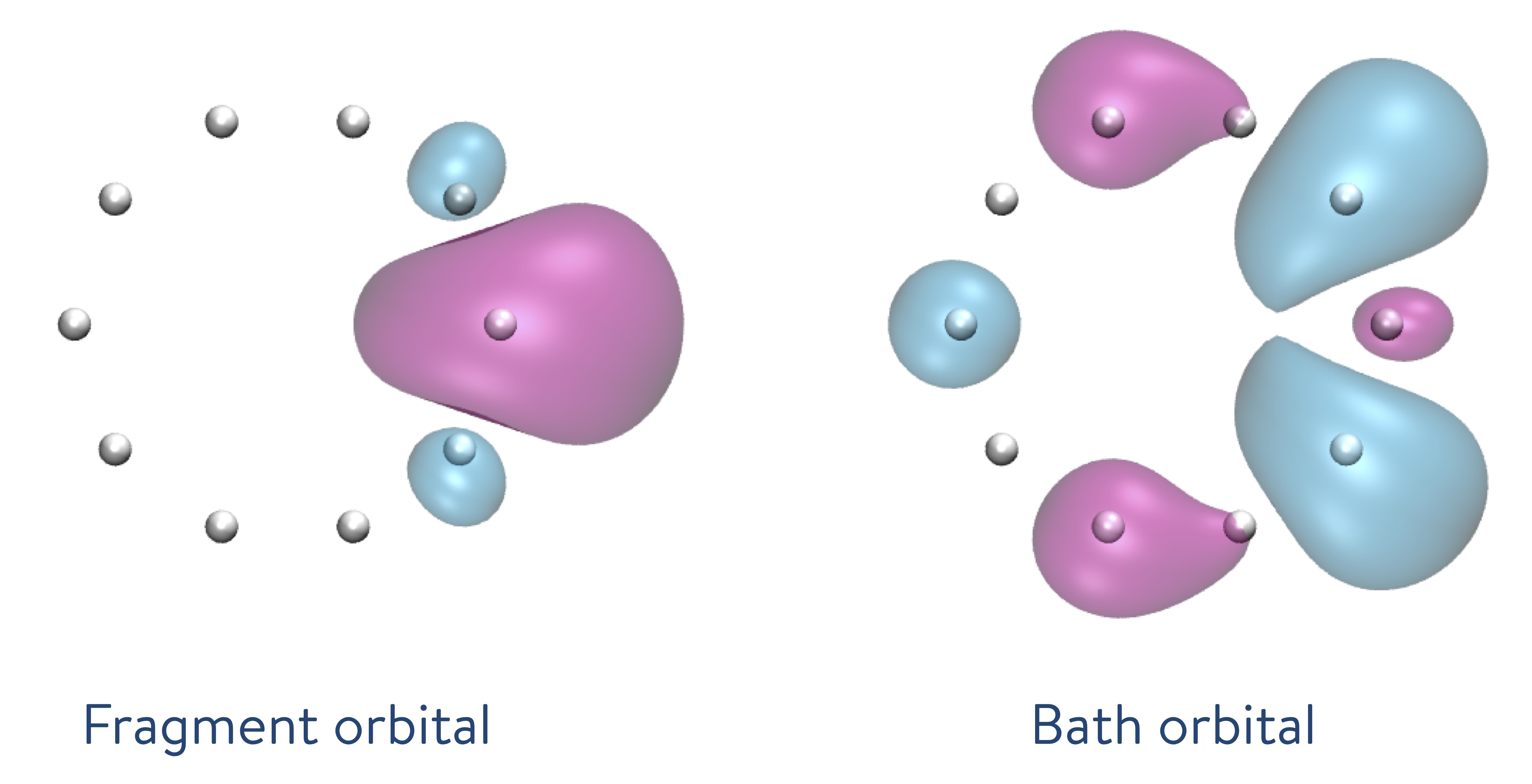
dmet_h10.build()The dmet.build() method creates fragments (10) from the H10 molecule. When we decompose the ring of atoms into fragments including only one hydrogen atom each, the DMET method creates a fragment orbital (left: the single orbital distribution is shown in both pink and blue, with the colours depicting the phases) and the bath orbital (right: the single orbital distribution of the remaining nine hydrogen atoms is shown in both pink and blue, with the colours depicting the phases).
Resource estimation is done by calling dmet_h10.get_resources(). Here, a list of ten dictionaries is returned and stored in resources_h10_dmet. Each dictionary refers to a fragment. As every fragment is the same in this system (a single hydrogen atom), we only print one.
resources_h10_dmet = dmet_h10.get_resources()
print(resources_h10_dmet[0])
{'qubit_hamiltonian_terms': 27, 'circuit_width': 4, 'circuit_depth': 100, 'circuit_2qubit_gates': 64, 'circuit_var_gates': 12, 'vqe_variational_parameters': 2}Compared to a direct VQE algorithm, those resources are greatly reduced: from 20 qubits down to only 4 qubits in our case. Below, dmet_h10.simulate() computes the DMET-VQE energy.
The options currently selected specify that VQE must be run for each fragment, at each iteration of DMET: as such, it may take 2-3 minutes for this cell to finish. The verbose option is turned off to hide the lengthy prints: feel free to turn it back on to track the progress of this cell, if you’d like.
dmet_h10.verbose = False
energy_h10_dmet = dmet_h10.simulate()

print(f"DMET energy (hartree): \t {energy_h10_dmet}")
DMET energy (hartree): -5.367548588351571A comparison with an FCI calculation is then made.
fci_h10 = FCISolver(mol_h10)
energy_h10_fci = fci_h10.simulate()

print(f"FCI energy (hartree): \t {energy_h10_fci}")
FCI energy (hartree): -5.3809260007310336Lastly, we note that the DMET energy is closer to the FCI energy than the HF energy. DMET-VQE results are an improvement but are still not at the FCI level. This discrepancy is attributable to missing three, four … many body interactions. When dismantling the system into fragments, we get a single hydrogen atom per fragment. Therefore, those fragments cannot propagate higher level (three and more) excitations. DMET user should have in mind this dilemma between fragment sizes and accuracy of the total electronic energy.
energy_h10_hf = dmet_h10.mean_field.e_tot
delta_h10_fci_hf = abs(energy_h10_fci - energy_h10_hf)
delta_h10_fci_dmet = abs(energy_h10_fci - energy_h10_dmet)

print(f"Difference FCI vs HF energies (hartree): \t\t {delta_h10_fci_hf}")
print(f"Difference FCI vs DMET-VQE energies (hartree): \t\t {delta_h10_fci_dmet}")
print(f"Difference FCI vs HF energies (kcal/mol): \t\t {627.5*delta_h10_fci_hf}")
print(f"Difference FCI vs DMET-VQE energies (kcal/mol): \t {627.5*delta_h10_fci_dmet}")
Difference FCI vs HF energies (hartree): 0.11680533556191364
Difference FCI vs DMET-VQE energies (hartree): 0.013377412379462328
Difference FCI vs HF energies (kcal/mol): 73.29534806510081
Difference FCI vs DMET-VQE energies (kcal/mol): 8.394326268112615. DMET features
In this section, some DMET features are shown. A four hydrogen atoms system is defined for this purpose.
H4 = """
H 0.7071 0. 0.
H 0. 0.7071 0.
H -1.0071 0. 0.
H 0. -1.0071 0.
"""

mol_h4 = SecondQuantizedMolecule(H4, q=0, spin=0, basis="3-21g")
5.1 Localization method
Electron localization is used to define the bath and the environment orbitals. There are two options available:
Localization.meta_lowdin(default): Described in Q. Sun et al., JCTC 10, 3784-3790 (2014).Localization.iao: Described in G. Knizia, JCTC 9, 4834-4843 (2013). This algorithm maps the orbitals to an minao set. So, at least a double zeta basis set must be used with this localization method.
options_h4_dmet = {"molecule": mol_h4,
                   "fragment_atoms": [1]*4,
                   "electron_localization": Localization.iao,
                   "verbose": False}

dmet_h4 = DMETProblemDecomposition(options_h4_dmet)
vars(dmet_h4)
{'molecule': <pyscf.gto.mole.Mole at 0x7efc9f011160>,
'electron_localization': <Localization.iao: 1>,
'fragment_atoms': [1, 1, 1, 1],
'fragment_solvers': ['ccsd', 'ccsd', 'ccsd', 'ccsd'],
'fragment_frozen_orbitals': [None, None, None, None],
'optimizer': <bound method DMETProblemDecomposition._default_optimizer of <tangelo.problem_decomposition.dmet.dmet_problem_decomposition.DMETProblemDecomposition object at 0x7efc9f0117c0>>,
'initial_chemical_potential': 0.0,
'solvers_options': [{}, {}, {}, {}],
'virtual_orbital_threshold': 1e-13,
'verbose': False,
'builtin_localization': {<Localization.iao: 1>,
<Localization.meta_lowdin: 0>,
<Localization.nao: 2>},
'fragment_builder': tangelo.problem_decomposition.dmet.fragment.SecondQuantizedDMETFragment,
'uhf': False,
'mean_field': <pyscf.scf.hf.RHF at 0x7efd0b4325b0>,
'chemical_potential': None,
'dmet_energy': None,
'orbitals': None,
'orb_list': None,
'orb_list2': None,
'onerdm_low': None,
'solver_fragment_dict': {},
'n_iter': 0}5.2 Fragment solvers
A list of solvers can be passed to the DMETProblemDecomposition class. If a single solver is detected, it will be applied to all fragments. Here is an example where the first fragment is solved with VQE, the second one with CCSD, the third one with FCI and the last one with VQE.
options_h4_dmet = {"molecule": mol_h4,
                   "fragment_atoms": [1]*4,
                   "fragment_solvers": ["vqe", "ccsd", "fci", "vqe"],
                   "verbose": False}

dmet_h4 = DMETProblemDecomposition(options_h4_dmet)
vars(dmet_h4)
{'molecule': <pyscf.gto.mole.Mole at 0x7efc9f136130>,
'electron_localization': <Localization.meta_lowdin: 0>,
'fragment_atoms': [1, 1, 1, 1],
'fragment_solvers': ['vqe', 'ccsd', 'fci', 'vqe'],
'fragment_frozen_orbitals': [None, None, None, None],
'optimizer': <bound method DMETProblemDecomposition._default_optimizer of <tangelo.problem_decomposition.dmet.dmet_problem_decomposition.DMETProblemDecomposition object at 0x7efce75930a0>>,
'initial_chemical_potential': 0.0,
'solvers_options': [{'qubit_mapping': 'jw',
'initial_var_params': 'ones',
'verbose': False},
{},
{},
{'qubit_mapping': 'jw', 'initial_var_params': 'ones', 'verbose': False}],
'virtual_orbital_threshold': 1e-13,
'verbose': False,
'builtin_localization': {<Localization.iao: 1>,
<Localization.meta_lowdin: 0>,
<Localization.nao: 2>},
'fragment_builder': tangelo.problem_decomposition.dmet.fragment.SecondQuantizedDMETFragment,
'uhf': False,
'mean_field': <pyscf.scf.hf.RHF at 0x7efd0b4325b0>,
'chemical_potential': None,
'dmet_energy': None,
'orbitals': None,
'orb_list': None,
'orb_list2': None,
'onerdm_low': None,
'solver_fragment_dict': {},
'n_iter': 0}5.3 Initial chemical potential
The DMET optimizes a parameter \(\mu\), the chemical potential. It ensures that the sum of all fragment electrons is consistent with the total number of electrons. As it is numerically optimized, the initial value can be important. Here is an example where the initial_chemical_potential is set to 0.1.
options_h4_dmet = {"molecule": mol_h4,
                   "fragment_atoms": [1]*4,
                   "initial_chemical_potential" : 0.1,
                   "verbose": False}

dmet_h4 = DMETProblemDecomposition(options_h4_dmet)
vars(dmet_h4)
{'molecule': <pyscf.gto.mole.Mole at 0x7efcf41d3130>,
'electron_localization': <Localization.meta_lowdin: 0>,
'fragment_atoms': [1, 1, 1, 1],
'fragment_solvers': ['ccsd', 'ccsd', 'ccsd', 'ccsd'],
'fragment_frozen_orbitals': [None, None, None, None],
'optimizer': <bound method DMETProblemDecomposition._default_optimizer of <tangelo.problem_decomposition.dmet.dmet_problem_decomposition.DMETProblemDecomposition object at 0x7efcf41d3190>>,
'initial_chemical_potential': 0.1,
'solvers_options': [{}, {}, {}, {}],
'virtual_orbital_threshold': 1e-13,
'verbose': False,
'builtin_localization': {<Localization.iao: 1>,
<Localization.meta_lowdin: 0>,
<Localization.nao: 2>},
'fragment_builder': tangelo.problem_decomposition.dmet.fragment.SecondQuantizedDMETFragment,
'uhf': False,
'mean_field': <pyscf.scf.hf.RHF at 0x7efd0b4325b0>,
'chemical_potential': None,
'dmet_energy': None,
'orbitals': None,
'orb_list': None,
'orb_list2': None,
'onerdm_low': None,
'solver_fragment_dict': {},
'n_iter': 0}5.4 Solvers options
A list of options can be passed to the solvers. Each element of the list must be consistent with the appropriate value in fragment_solvers. If a single dictionary of options is detected, it is applied to all fragment solvers. Here is an example where one wants to set the qubit mapping to the Bravyi-Kitaev method when performing VQE.
vqe_options = {"qubit_mapping": "bk"}

options_h4_dmet = {"molecule": mol_h4,
                   "fragment_atoms": [1]*4,
                   "fragment_solvers": "vqe",
                   "solvers_options": vqe_options,
                   "verbose": False}

dmet_h4 = DMETProblemDecomposition(options_h4_dmet)
vars(dmet_h4)
{'molecule': <pyscf.gto.mole.Mole at 0x7efc9f136a60>,
'electron_localization': <Localization.meta_lowdin: 0>,
'fragment_atoms': [1, 1, 1, 1],
'fragment_solvers': ['vqe', 'vqe', 'vqe', 'vqe'],
'fragment_frozen_orbitals': [None, None, None, None],
'optimizer': <bound method DMETProblemDecomposition._default_optimizer of <tangelo.problem_decomposition.dmet.dmet_problem_decomposition.DMETProblemDecomposition object at 0x7efc9f136700>>,
'initial_chemical_potential': 0.0,
'solvers_options': [{'qubit_mapping': 'bk'},
{'qubit_mapping': 'bk'},
{'qubit_mapping': 'bk'},
{'qubit_mapping': 'bk'}],
'virtual_orbital_threshold': 1e-13,
'verbose': False,
'builtin_localization': {<Localization.iao: 1>,
<Localization.meta_lowdin: 0>,
<Localization.nao: 2>},
'fragment_builder': tangelo.problem_decomposition.dmet.fragment.SecondQuantizedDMETFragment,
'uhf': False,
'mean_field': <pyscf.scf.hf.RHF at 0x7efd0b4325b0>,
'chemical_potential': None,
'dmet_energy': None,
'orbitals': None,
'orb_list': None,
'orb_list2': None,
'onerdm_low': None,
'solver_fragment_dict': {},
'n_iter': 0}5.5 Restricting the fragment active space
Problem decomposition is successful at reducing the problem size, but the subproblems still can demand too much resources for a quantum computer. It is possible to define an active space in each DMET fragment, and an example is shown below.
def define_dmet_frag_as(homo_minus_m=0, lumo_plus_n=0):
    def callable_for_dmet_object(info_fragment):
        mf_fragment, _, _, _, _, _, _ = info_fragment

        n_molecular_orb = len(mf_fragment.mo_occ)

        n_lumo = mf_fragment.mo_occ.tolist().index(0.)
        n_homo = n_lumo - 1

        frozen_orbitals = [n for n in range(n_molecular_orb) if n not in range(n_homo-homo_minus_m, n_lumo+lumo_plus_n+1)]

        return frozen_orbitals

    return callable_for_dmet_object

options_h4_dmet = {"molecule": mol_h4,
                   "fragment_atoms": [1]*4,
                   # The fragment active space can be selected with a nested list on ints (corresponding
                   # to orbital indices), or a function.
                   "fragment_frozen_orbitals": [define_dmet_frag_as(0, 0), [0, 3, 4], define_dmet_frag_as(1, 1), None],
                   "fragment_solvers": "vqe",
                   "solvers_options": vqe_options,
                   "verbose": False}

dmet_h4 = DMETProblemDecomposition(options_h4_dmet)
dmet_h4.build()

# Use json to make the print format more readable
print(json.dumps(dmet_h4.get_resources(), indent=2))
{
"0": {
"qubit_hamiltonian_terms": 27,
"circuit_width": 4,
"circuit_depth": 76,
"circuit_2qubit_gates": 46,
"circuit_var_gates": 12,
"vqe_variational_parameters": 2
},
"1": {
"qubit_hamiltonian_terms": 27,
"circuit_width": 4,
"circuit_depth": 76,
"circuit_2qubit_gates": 46,
"circuit_var_gates": 12,
"vqe_variational_parameters": 2
},
"2": {
"qubit_hamiltonian_terms": 361,
"circuit_width": 8,
"circuit_depth": 1573,
"circuit_2qubit_gates": 1180,
"circuit_var_gates": 160,
"vqe_variational_parameters": 14
},
"3": {
"qubit_hamiltonian_terms": 361,
"circuit_width": 8,
"circuit_depth": 1573,
"circuit_2qubit_gates": 1180,
"circuit_var_gates": 160,
"vqe_variational_parameters": 14
}
}6. Closing words
This concludes our overview of DMETProblemDecomposition. There are many flavors of DMET and only one has been discussed here. Here we refer some papers relevant for the reader who wants more details:
Theory
- S. Wouters, C.A. Jiménez-Hoyos, Q. Sun, and G.K.L. Chan, J. Chem. Theory Comput. 12, 2706 (2016).
- G. Knizia and G.K.L. Chan, J. Chem. Theory Comput. 9, 1428 (2013).
- G. Knizia and G.K.L. Chan, Phys. Rev. Lett. 109, 186404 (2012).
Good Chemistry Company papers on the subject
- Y. Kawashima, M.P. Coons, Y. Nam, E. Lloyd, S. Matsuura, A.J. Garza, S. Johri, L. Huntington, V. Senicourt, A.O. Maksymov, J.H. V. Nguyen, J. Kim, N. Alidoust, A. Zaribafiyan, and T. Yamazaki, ArXiv:2102.07045 (2021).
- T. Yamazaki, S. Matsuura, A. Narimani, A. Saidmuradov, and A. Zaribafiyan, ArXiv:1806.01305 (2018).