# If Tangelo is not found in your current environment, this cell installs all dependencies required for this hands-on
try:
    import tangelo
except ModuleNotFoundError:
    !pip install git+https://github.com/sandbox-quantum/Tangelo.git@develop  --quiet
!pip install pyscf --quietFault Tolerant Building blocks
Before you jump in
This hands-on notebook complements existing tutorials, documentation and the developer notes available in the Tangelo GitHub repositories, which present content in much more depth.
You will come across code cells that require you to change code or fill in the blanks in order to achieve a desired outcome. There may be many ways to solve these small exercises, and you are encouraged to explore.
In order to complete this hands-on tutorial, we recommend you install the latest version of Tangelo. If you encounter errors related to missing Python packages (classical chemistry backend, quantum circuit simulator…), you can install them on-the-fly by typing !pip install <package-name> in a new code cell, and then restart the Jupyter notebook kernel.
For this hands-on, we recommend the following resources: - the first part of this tutorial notebook on linq, about gates and circuits. - the documentation for the Gate (here) and Circuit (here) classes.
Hands-On
Unlike NISQ algorithms which utilize shallow circuits and require many measurements, fault-tolerant algorithms rely on deeper circuits and fewer measurements. The quantum computer can efficiently store large (exponential) systems efficiently but preparing these states is time-consuming and we generally don’t need all the information about the state.
1. Controlled Operations
A main component of fault-tolerant algorithms is controlled operations. These are defined such that operations given a state of a certain (set of) qubit(s), one can apply an operation to a different set of qubits. For example, the usual CNOT (CX) Gate applies X to the target qubit only if the control qubit is in the \(\big|1\big>\) state, and does nothing otherwise. This can be written as
\(CX\big|0\big>\big|s\big>=\big|0\big>\big|s\big>, \quad CX\big|1\big>\big|s\big>=\big|1\big>X\big|s\big>\) where \(s\) is any single-qubit state \(a\big|0\big> + b\big|1\big>\).
Likewise, this can be generalized to multiple controlled operations. For example, if we want to apply an operation \(U\) only when the first 2-qubits are in state \(|1\rangle\). We can define
\(C_{11}U\big|11\big>\big|s\big>=\big|11\big>U\big|s\big>, \quad C_{11}U\big|10\big>\big|s\big>=\big|10\big>\big|s\big>, \quad C_{11}U\big|01\big>\big|s\big>=\big|01\big>\big|s\big>, \quad C_{00}U\big|00\big>\big|s\big>=\big|00\big>\big|s\big>\)
Where the subscript \((11)\) on the \(C\) indicates that the first two qubits should be in state \(|1\rangle\). In general the operation can be controlled on many qubits and \(s\) can be a many-qubit state.
from itertools import product
from tangelo.linq import Circuit, Gate, get_backend

# We use a cirq backend as the ordering of the statevector is the same as qubit operators, currently from Openfermion
sim = get_backend("cirq")
Q: Can you fill in the blanks in the cell below, to run the algorithm for a controlled-X gate? In Tangelo, adding “C” in front of the gate’s name indicates that a controlled operation is requested.
# INSERT YOUR CODE HERE
cx = Gate("CX", 1, control=[0])

# Run through all possible combinations of inputs and print the result
c0 = Circuit([cx])
c1 = Circuit([Gate("X", 0), cx])
print(f"If qubit 0 is in state '0' then the frequencies are {sim.simulate(c0)[0]}")
print(f"If qubit 0 is in state '1' then the frequencies are {sim.simulate(c1)[0]}")
If qubit 0 is in state '0' then the frequencies are {'00': 1.0}
If qubit 0 is in state '1' then the frequencies are {'11': 1.0}Q: Can you apply the operation controlled on qubits 1 and 2, such that the first qubit flips to state “1” only if qubits 1 and and 2 are in state “1” ? The \(C_{11}X\) operation is also known as the Toffoli gate.
# INSERT YOUR CODE HERE
ccx = Gate("CX", 2, control=[0, 1])

# Run through all possible combinations of inputs and print the result
c00 = Circuit([ccx])
c10 = Circuit([Gate("X", 0), ccx])
c01 = Circuit([Gate("X", 1), ccx])
c11 = Circuit([Gate("X", 0), Gate("X", 1), ccx])
print(f"If qubits [0,1] are in state '00' then the frequencies are {sim.simulate(c00)[0]}")
print(f"If qubits [0,1] are in state '10' then the frequencies are {sim.simulate(c01)[0]}")
print(f"If qubits [0,1] are in state '01' then the frequencies are {sim.simulate(c10)[0]}")
print(f"If qubits [0,1] are in state '11' then the frequencies are {sim.simulate(c11)[0]}")
If qubits [0,1] are in state '00' then the frequencies are {'000': 1.0}
If qubits [0,1] are in state '10' then the frequencies are {'010': 1.0}
If qubits [0,1] are in state '01' then the frequencies are {'100': 1.0}
If qubits [0,1] are in state '11' then the frequencies are {'111': 1.0}If one wants to apply the operation \(C_{10}X\). The same operations can be used but sandwiched with \(X\) gates. We flip second qubit using an \(X\big|0\big>=\big|1\big>\) operation, apply the \(ccx\) operation and apply \(X\big|1\big>=\big|0\big>\) on the second qubit again. You can run the code below to obtain the same result.
flip_2nd_qubit = Gate("X", 1)

# Run through all possible combinations of inputs and print the result
c00 = Circuit([flip_2nd_qubit, ccx, flip_2nd_qubit])
c10 = Circuit([Gate("X", 0), flip_2nd_qubit, ccx, flip_2nd_qubit])
c01 = Circuit([Gate("X", 1), flip_2nd_qubit, ccx, flip_2nd_qubit])
c11 = Circuit([Gate("X", 0), Gate("X", 1), flip_2nd_qubit, ccx, flip_2nd_qubit])
print(f"If qubits [0,1] are in state '00' then the frequencies are {sim.simulate(c00)[0]}")
print(f"If qubits [0,1] are in state '10' then the frequencies are {sim.simulate(c01)[0]}")
print(f"If qubits [0,1] are in state '01' then the frequencies are {sim.simulate(c10)[0]}")
print(f"If qubits [0,1] are in state '11' then the frequencies are {sim.simulate(c11)[0]}")
If qubits [0,1] are in state '00' then the frequencies are {'000': 1.0}
If qubits [0,1] are in state '10' then the frequencies are {'010': 1.0}
If qubits [0,1] are in state '01' then the frequencies are {'101': 1.0}
If qubits [0,1] are in state '11' then the frequencies are {'110': 1.0}We successfully applied the operation \(C_{01}X\) using the same \(CCX\) gate you defined above.
In general, we can make more complicated controlled unitaries. For instance, we could implement quantum phase estimation, one of the key fault-tolerant algorithms. Using a series of controlled operations followed by a Quantum Fourier Transform (QFT), this algorithm can approximate the eigenvalues of a state.
2. Quantum Phase Estimation
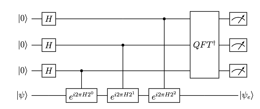
The first fault-tolerant algorithm we look at in is quantum phase-estimation (QPE). It is a technique to obtain the energy (E) of an eigenstate \(\big|\psi_e\big>\) of a Hamiltonian defined \(H\big|\psi_e\big>=E\big|\psi_e\big>\). The energy is a very important quantity to know in chemistry as it determines how chemistry happens from chemical reactions to light-matter interactions.
The input is an approximate eigenstate \(\big|\psi_e\big>\). QPE then utilizes a series of controlled time-evolutions of a Hamiltonian on different qubits followed by the quantum version of the Fourier Transform (i.e. Quantum Fourier Transform (QFT)). The circuit is shown below:
Tangelo provides a
QPESolverclass allowing you to simulate QPE with built-in and user-defined unitaries, for time-evolution. If you are already familiar withVQESolverthen its interface should feel straightforward. We illustrate this ready-made QPE framework briefly at the end of the section. The first part of this section of the hands-on however offers to retrace the steps taken to implement such fault-tolerant algorithms, and manipulating advanced building-blocks (controlled unitaries, trotterization, QFT, circuit inverses, simulation with desired measurements …).
a) Building QPE from “scratch” with fault-tolerant building blocks
For our use case, we first generate the qubit Hamiltonian for molecular Hydrogen (\(H_2\)) in a STO-3G basis. To show the algorithm is working as expected, we calculate all the eigenstates and select the two singlet states with 2 electrons. This is not possible for much larger systems but we can extrapolate the success demonstrated here to show that we can obtain good results.
import numpy as np
from openfermion import get_sparse_operator

from tangelo.molecule_library import mol_H2_sto3g
from tangelo.toolboxes.qubit_mappings.mapping_transform import fermion_to_qubit_mapping
from tangelo.toolboxes.qubit_mappings.statevector_mapping import get_reference_circuit

# Qubit operator representing H2 in a minimal basis
mol = mol_H2_sto3g
qu_op = fermion_to_qubit_mapping(mol.fermionic_hamiltonian, mapping="JW",
                                 n_spinorbitals=mol.n_active_sos, n_electrons=mol.n_active_electrons,
                                 spin=mol.spin, up_then_down=False)

# Shift ground state eigenvalue to be 0.25, such that a short-time QPE can return the exact energy
# (the exact ground state energy is known to be 1.137270174660903)
qu_op += (0.25 + 1.137270174660903)
eigs, eigenstates = np.linalg.eigh(get_sparse_operator(qu_op).toarray())

# When converting from a Fermion Hamiltonian to an Qubit Hamiltonian, a bunch of physical but not desired eigenstates are obtained
# We are looking for the ground and first excited Singlet S^2 states.
ground_sv = eigenstates[:, 0]
first_sv = eigenstates[:, 13]
/Users/valentinsenicourt/Desktop/virtualenvs/hands_on/lib/python3.10/site-packages/pyscf/dft/libxc.py:772: UserWarning: Since PySCF-2.3, B3LYP (and B3P86) are changed to the VWN-RPA variant, the same to the B3LYP functional in Gaussian and ORCA (issue 1480). To restore the VWN5 definition, you can put the setting "B3LYP_WITH_VWN5 = True" in pyscf_conf.py
warnings.warn('Since PySCF-2.3, B3LYP (and B3P86) are changed to the VWN-RPA variant, 'In order to compare how close the initial approximate state is to the exact eigenstate, we are going to use the overlap (dot product) between the states. If the overlap is 1 then the states are equivalent.
# Hartree-Fock reference state circuit
hf_circuit = get_reference_circuit(n_spinorbitals=mol.n_active_sos, n_electrons=mol.n_active_electrons, mapping="JW",
                                   up_then_down=False, spin=mol.spin)
f, hf_sv = sim.simulate(hf_circuit, return_statevector=True)

# Dot product to compare how close the initial Hartree-Fock reference is to the ground and first excited singlet state.
g_ovlp = np.dot(hf_sv, ground_sv)
f_ovlp = np.dot(hf_sv, first_sv)
print(f"The overlap of the initial (Hartree-Fock) state with the exact ground state is        {g_ovlp}")
print(f"The overlap of the initial (Hartree-Fock) state with the exact first excited state is {f_ovlp}")
The overlap of the initial (Hartree-Fock) state with the exact ground state is (0.9936146058054715+0j)
The overlap of the initial (Hartree-Fock) state with the exact first excited state is (-0.11282736871006808+0j)Q: Can you fill in the blanks in the cell below, to run the algorithm originally illustrated in the circuit diagram ? It should return
"010"with very-high probability (~98%), corresponding to an energy of 0.25. You may need to change the parameters used in the Trotter-Suzuki (trotterize) operation to obtain accurate enough time-evolution to get a good result.
from tangelo.toolboxes.ansatz_generator.ansatz_utils import trotterize, get_qft_circuit
from tangelo.toolboxes.post_processing.histogram import Histogram

# Reverse order as cirq uses lsq_first
qubit_list = [6, 5, 4]

# State preparation
pe_circuit = hf_circuit + Circuit([Gate("H", q) for q in qubit_list])

for i, qubit in enumerate(qubit_list):
    # INSERT CODE HERE
    # You can play around with how accurate the time-evolution needs to be
    # Use negative time as trotterize uses exp(-iHt) to follow the Schrodinger equation
    pe_circuit += trotterize(qu_op, trotter_order=4, n_trotter_steps=12, time=-2*np.pi*2**i, control=qubit)

# INSERT CODE HERE
# Set inverse to true or false
pe_circuit += get_qft_circuit(qubit_list, inverse=True)
freqs, _ = sim.simulate(pe_circuit)

# Remove qubit indices from histogram corresponding to the state qubits i.e. (0, 1, 2, 3)
hist = Histogram(freqs)
hist.remove_qubit_indices(0, 1, 2, 3)

for key, probability in hist.frequencies.items():
      energy = sum(int(k)/2**(i+1) for i, k in enumerate(key))
      print(f"The measurement {key} with probability {probability:3.5f} converts to an energy={energy} ")
The measurement 000 with probability 0.00004 converts to an energy=0.0
The measurement 001 with probability 0.00001 converts to an energy=0.125
The measurement 010 with probability 0.98752 converts to an energy=0.25
The measurement 011 with probability 0.00005 converts to an energy=0.375
The measurement 100 with probability 0.00001 converts to an energy=0.5
The measurement 101 with probability 0.00003 converts to an energy=0.625
The measurement 110 with probability 0.00005 converts to an energy=0.75
The measurement 111 with probability 0.01228 converts to an energy=0.875 In Tangelo, simulators can take the option desired_measurement to return the quantum state corresponding to the state preparation done under specific values of measurement gates. Assuming you are interested in a specific outcome - "010" for our use case - we can retrieve both the probability that such measurements are observed, and the corresponding quantum state and compute its overlap with the ground state:
desired_measurement = "010"
pe_plus_measure = pe_circuit + Circuit([Gate("MEASURE", i) for i in qubit_list])
_, sv_new = sim.simulate(pe_plus_measure, desired_meas_result=desired_measurement, return_statevector=True)
print(f"The probability of this measurement is {pe_plus_measure.success_probabilities[desired_measurement]}")
# Shrink vector down to 2**4 size to compare with exact ground state.
sv_new_post = np.reshape(sv_new, (2**4, 2**3))[:, int(desired_measurement, base=2)]
print(f"The final state overlap with the ground state is {np.abs(np.dot(sv_new_post, ground_sv))}")The probability of this measurement is 0.9875184986388712
The final state overlap with the ground state is 0.999972738775133We can see that we measured the desired energy with probability 0.987 and the resulting state has overlap with the exact state of 0.99997, while we originally started with an overlap of 0.9936. We not only measured the energy of an eigenstate, we also created the eigenstate on the simulator. This eigenstate can then be used to perform other tasks!
Q: By using the previous cell as an example, can you look into what happens for “111”, which is close to the energy of the first excited singlet state?
# INSERT CODE HERE
desired_measurement = "111"
pe_plus_measure = pe_circuit + Circuit([Gate("MEASURE", i) for i in qubit_list])
_, sv_new = sim.simulate(pe_plus_measure, desired_meas_result=desired_measurement, return_statevector=True)
print(f"The probability of this measurement is {pe_plus_measure.success_probabilities[desired_measurement]}")
# Shrink vector down to 2**4 size to compare with exact ground state.
sv_new_post = np.reshape(sv_new, (2**4, 2**3))[:, int(desired_measurement, base=2)]
print(f"The final state overlap with the first excited singlet state is {np.abs(np.dot(sv_new_post, first_sv))}")The probability of this measurement is 0.012282064140958449
The final state overlap with the first excited singlet state is 0.9998680358098742We can see that starting with the same Hartree-Fock reference state, we obtained a good approximation (\(>0.999\)) overlap to the first excited singlet state when measuring a result close to the exact energy with very low probability (around 1%). Also, the energy we obtained \(0.875\) is not chemically accurate (\(<0.001\) Hartree error). We can only obtain energies mod 1 and the exact energy is \(1.867\) so the error is \(0.008\).
However, even this is fortunate. To ensure we obtain chemical accuracy, we would need to run the algorithm with 7 ancilla qubits \(1/2^7\approx 0.008\). This would require time-evolution that is about 16 times longer that what we ran above.
b) Ready-made QPESolver framework
Tangelo provides a QPESolver class allowing you to simulate QPE with built-in and user-defined unitaries, for time-evolution. If you are already familiar with VQESolver then its interface should feel straightforward (instantiate with options, build, simulate, get_resources). You can check out the source code in the tests in Tangelo to see how one could provide a molecule, or built-in unitaries. Below, we reproduce the work done in the previous section by directly passing the qubit Hamiltonian we obtained for \(H_2\) earlier.
from tangelo.algorithms.projective.qpe import QPESolver
qpe_solver = QPESolver({"qubit_hamiltonian": qu_op, "size_qpe_register": 3, "ref_state": hf_circuit, "backend_options": {"target": "cirq"},
"unitary_options": {"time": -2*np.pi, "n_trotter_steps": 12, "n_steps_method": "time", "trotter_order": 4}})
qpe_solver.build()
energy = qpe_solver.simulate()
print(f"QPESolver returned an energy of {energy}")
for key, probability in qpe_solver.qpe_freqs.items():
energy = sum(int(k)/2**(i+1) for i, k in enumerate(key))
print(f"The measurement {key} with probability {probability:3.5f} converts to an energy={energy} ")QPESolver returned an energy of 0.25
The measurement 000 with probability 0.00004 converts to an energy=0.0
The measurement 001 with probability 0.00001 converts to an energy=0.125
The measurement 010 with probability 0.98752 converts to an energy=0.25
The measurement 011 with probability 0.00005 converts to an energy=0.375
The measurement 100 with probability 0.00001 converts to an energy=0.5
The measurement 101 with probability 0.00003 converts to an energy=0.625
The measurement 110 with probability 0.00005 converts to an energy=0.75
The measurement 111 with probability 0.01228 converts to an energy=0.875 Much simpler, isn’t it ? If you would like to see more fault-tolerant algorithms available “out of the box” in Tangelo, please consider contributing to the project or put a feature request on GitHub.
3 .Block encodings.
Another building block of many fault-tolerant algorithms is block encodings. This is a technique to implement any operation as long as it can be decomposed into a linear combination of Unitaries. We can implement the operation using \(U_{prep}\) and \(U_{select}\) defined for a general operator \(A=\sum_i c_i U_i\) where \(U_i\) are unitaries.
\(U_{prep}\big|\psi\big>\big|0\big> = \sum_{i}\sqrt{\frac{|c_i|}{\alpha}}\big|\psi\big>\big|i\big>\)
\(U_{select}\big|\psi\big>\big|i\big> = U_i\big|\psi\big>\big|i\big>\)
where \(\alpha\) is the 1-norm of the coefficients \(|c_i|\)
Applying the circuit \(U_{prep}U_{select}U_{prep}^{\dagger}\) results in \(A\big|\psi\big>\big|0\big> + \sum_i \big|\psi^{\perp}\big>\big|i\big>\) where \(\psi^{\perp}\) are states orthogonal to \(A\psi\). This means that if we measure the ancilla qubits and the result is zero, we have successfully applied the desired operation \(A\).
For example, let’s try to apply \(A=\frac{1}{\sqrt{2}}X+\frac{1}{\sqrt{2}}Y\) which is equivalent to \(\left[\begin{array}{cc}0&\frac{1-i}{\sqrt{2}}\\ \frac{1+i}{\sqrt{2}}&0\end{array}\right]\)
from tangelo.toolboxes.operators import QubitOperator
from tangelo.linq.helpers.circuits.statevector import StateVector

coefs = [1/np.sqrt(2), 1/np.sqrt(2)]
a = QubitOperator("X0", coefs[0]) + QubitOperator("Y0", coefs[1])

vec = np.array(np.abs(coefs))
vec = np.sqrt(vec/np.sum(vec))

# In this case prep can be be applied by simply applying the Hadamard gate to the first qubit
uprep = Circuit([Gate("H", 1)])

sv = StateVector(vec)
uprep = sv.initializing_circuit()
uprep.reindex_qubits([1])
Q: Can you fill in the blanks in the cell below, to apply the \(U_{select}\) operation \(A\) defined as a linear combination of unitaries \(X\) and \(Y\) ?
# INSERT YOUR CODE HERE

# Qubit 1 is the "prep" register with coefficients [1/sqrt(2), 1/sqrt(2)]
cy1 = [Gate("CY", target=0, control=1)]
# Sandwiching with "X" gates flips the control bit such that operation is controled on state "0"
cx0 = [Gate("X", 1), Gate("CX", target=0, control=1), Gate("X", 1)]
We can now run the block-encoded circuit. If your code is correct, it will return the correct state with probability 0.5 and the overlap will be 1.
# Uselect
uselect = Circuit(cx0 + cy1)

# We will use this as a state prep circuit. You can change this to any set of operations on qubit 0
state_prep = Circuit([Gate("RY", 0, parameter=np.pi/4)])

_, init_state = sim.simulate(state_prep, return_statevector=True)
block_circuit = uprep + uselect + uprep.inverse()
circuit = state_prep + block_circuit + Circuit([Gate("MEASURE", 1)])

desired_measurement = "0"
f, sv = sim.simulate(circuit, desired_meas_result=desired_measurement, return_statevector=True)
final_state = sv.reshape(2,2)[:,int(desired_measurement, base=2)]
print(f"The success probability of the operation was {circuit.success_probabilities['0']}")

final_exact = get_sparse_operator(a).toarray() @ init_state
final_exact /= np.linalg.norm(final_exact)

print(f"The overlap of the exact with the block encoded application of A is {np.abs(np.vdot(final_state, final_exact))}")
The success probability of the operation was 0.4999999999999999
The overlap of the exact with the block encoded application of A is 1.04. Amplitude Amplification
We would like to have a higher probability of success than 0.5. This is the main point of Grover’s search where \(\sqrt{N}\) amplifications of the desired “good” state is required to increase the probability by \(N\). Hence, the quadratic speed up. To implement this we need to apply signed operations. However, we are going to implement the generalized Amplitude Amplification which is defined by the following circuit,
\(F_{good} F_{full}\),
where \(F_{good} = (1-\big|0\big>^{ancilla}\big<0\big|^{ancilla})\) and \(F_{full} = (1-A\big|\psi\big>\big<\psi\big|A)\) are in general (non-unitary operations).
For the purposes of applying \(A=\frac{1}{\sqrt{2}}X+\frac{1}{\sqrt{2}}Y\), the “good” subspace is all zeros on the ancilla qubits and the “full” state is the application of the state preparation and the \(A\) block encoding.
In order to facilitate amplitude amplification, we are going to make the 1-norm of the operator 2 such that the success probability is 25%. In order to facilitate this, the operator being applied is \((I - I + X + Y)\) which as \(\big|\big| A \big|\big|_1=2\) and the probability of success is \(1/\left(\big|\big| A \big|\big|_1\right)^4\). After one application of amplitude amplification, the operator will be applied with 100% probability.
Note: The “trick” of adding and subtracting terms proportional to the identity operator is common in fault-tolerant algorithms to obtain a circuit that has a success probability close to 100%.
from tangelo.toolboxes.circuits.lcu import sign_flip, get_uprep_uselect

# Generate operator and make 1-norm equal to 2 to ensure that the operation applies with 100% success
uprep, uselect, state_qubits, ancilla_qubits, alpha = get_uprep_uselect(a, make_alpha_eq_2=True)

def flip_on_state(qubits: list, circuit: Circuit):
    return circuit.inverse() + sign_flip(qubits) + circuit

block_circuit = uprep + uselect + uprep.inverse()
full_circuit = state_prep + block_circuit
Q: Can you fill in the blanks in the cell below to define the appropriate qubits and operation that the sign flip operations are applied to ? Remember that the amplifying circuit is \(F_{good}F_{full}\). Which qubits and what circuit generates the “good” \(|0\big>^{ancilla}\) state? Which qubits and what circuit generates the “full” \(A|\psi\big>\)?
# INSERT YOUR CODE HERE
amplifying_circuit = flip_on_state(ancilla_qubits, Circuit()) + flip_on_state(state_qubits+ancilla_qubits, full_circuit)
We can now check when comparing the unamplified circuit and the amplified circuit that the resulting statevector is the same (i.e. overlap is still 1) but the probability of success is 100%.
unamplified_circuit = state_prep + block_circuit + Circuit([Gate("MEASURE", q) for q in ancilla_qubits])
amplified_circuit = state_prep + block_circuit + amplifying_circuit + Circuit([Gate("MEASURE", q) for q in ancilla_qubits])

f, sv = sim.simulate(amplified_circuit, return_statevector=True, desired_meas_result="0"*len(ancilla_qubits))
amplified_final_state = sv.reshape(2,4)[:,0]
f, sv = sim.simulate(unamplified_circuit, return_statevector=True, desired_meas_result="0"*len(ancilla_qubits))
unamplified_final_state = sv.reshape(2,4)[:,0]
print(f"The overlap of the two states are {np.abs(np.vdot(amplified_final_state, unamplified_final_state)): 3.2f}")
print(f"The success probability has been increased from {unamplified_circuit.success_probabilities['00']: 3.2f} to "
      f"{amplified_circuit.success_probabilities['00']: 3.2f} after amplitude amplification")
print(f"The overlap of the amplified state with the exact state is {np.abs(np.vdot(final_state, amplified_final_state)): 3.2f}")
The overlap of the two states are 1.00
The success probability has been increased from 0.25 to 1.00 after amplitude amplification
The overlap of the amplified state with the exact state is 1.00Final Words
After this hands-on, you learned some of the building blocks of fault tolerant algorithms. You now understand how one utilizes controlled operations to obtain interesting information about a system (namely energy using QPE). You also learned about block-encodings which allow you to apply any operation probabilistically. Finally you learned about how to increase the probability of success using amplitude amplification.
If you are interested in contributing ready-made versions of fault-tolerant algorithms to the project, please do not hesitate !
Here are some additional material implementing some other fault-tolerant approaches which may be relevant to you: * Block encoding used for state preparation through Quantum Signal Processing. * More QPESolver examples * AWS Blog post that features a fault-tolerant simulation of a wavepacket